
First of all, I would like to express my sincere gratitude to the competition organizers for hosting this exciting challenge. Thanks to their efforts, I had the opportunity to learn a lot and improve my skills. I also appreciate the Kaggle community for their insightful discussions and valuable resources.
\nIn particular, I found @hengck23's discussions and notebooks extremely helpful. The insights and contributions were instrumental in shaping my approach to this competition.
sliding_window_inference to divide the input volume into fixed-size subvolumes and perform inference with 10 different models. Each model predicts a map for each particle type, indicating the locations of particles.
I utilized a 2.5D UNet based on this notebook, as well as MONAI’s 3D UNet and SegResNet. For the 2.5D UNet, timm's EfficientNet-B2, EfficientNetV2-B2, ConvNeXt-Nano, and ResNet34d were used as encoders. While the 3D UNet and SegResNet initially struggled to achieve good performance using only the training dataset, they reached a similar level of accuracy as the 2.5D UNet after pretraining on simulated data, which I will describe later.
\nTo improve model diversity, I trained a total of 10 models with slight variations in pretraining strategies, data augmentation techniques, and other hyperparameters. For the final submission, I used models trained on the entire training dataset.
As a preprocessing step, I first removed outliers and then applied min-max normalization. The input volumes were cropped to a fixed size of 64×128×128.
\nFor the training labels, I generated binary masks centered around each particle’s location. Specifically, I set the region within radius × 0.5 to 1 and all other areas to 0. I created these masks separately for each particle.
\nInitially, I experimented with BCE and Focal Loss, but these loss functions resulted in extremely slow convergence, likely due to the severe class imbalance. I then tried Dice Loss and Tversky Loss, which significantly accelerated training. However, these loss functions caused the model’s predictions to become overly binary, outputting only extreme values of 0 or 1.
\nSince my pipeline ensembles prediction maps by averaging them and then applies a threshold for binarization, such prediction values were undesirable. To address this, I used FocalTversky++ loss as proposed in this paper. By using this loss, the model outputs prediction maps that reflect its confidence.

I generated my own simulated data using polnet and used it to pretrain some of the models. To enhance the model’s ability to distinguish particles, I designed the simulated data to include particles with shapes similar to those of the target particles in this competition.
\n
For inference, I used MONAI’s sliding_window_inference with an overlap ratio of 0.25. Since predictions near the edges of subvolumes tend to be less stable, I discarded the outermost 8% of predictions to improve reliability.
\nI felt that one of the key challenges in this competition was achieving fast inference. To optimize speed, I first converted the models to TensorRT in a separate notebook before submission. During inference, I loaded the pre-converted TensorRT models and leveraged parallel processing with two T4 GPUs.
Once the ensembled prediction maps were obtained, I binarized them using particle-specific thresholds. These thresholds were initially estimated through cross-validation and later fine-tuned based on leaderboard.
\nAfter binarization, I performed connected component analysis on the binary map and extracted the centroid of each connected component as the particle location.
First of all, I would like to express my sincere gratitude to the competition organizers for hosting this exciting challenge. Thanks to their efforts, I had the opportunity to learn a lot and improve my skills. I also appreciate the Kaggle community for their insightful discussions and valuable resources.
\nIn particular, I found @hengck23's discussions and notebooks extremely helpful. The insights and contributions were instrumental in shaping my approach to this competition.
sliding_window_inference to divide the input volume into fixed-size subvolumes and perform inference with 10 different models. Each model predicts a map for each particle type, indicating the locations of particles.
I utilized a 2.5D UNet based on this notebook, as well as MONAI’s 3D UNet and SegResNet. For the 2.5D UNet, timm's EfficientNet-B2, EfficientNetV2-B2, ConvNeXt-Nano, and ResNet34d were used as encoders. While the 3D UNet and SegResNet initially struggled to achieve good performance using only the training dataset, they reached a similar level of accuracy as the 2.5D UNet after pretraining on simulated data, which I will describe later.
\nTo improve model diversity, I trained a total of 10 models with slight variations in pretraining strategies, data augmentation techniques, and other hyperparameters. For the final submission, I used models trained on the entire training dataset.
As a preprocessing step, I first removed outliers and then applied min-max normalization. The input volumes were cropped to a fixed size of 64×128×128.
\nFor the training labels, I generated binary masks centered around each particle’s location. Specifically, I set the region within radius × 0.5 to 1 and all other areas to 0. I created these masks separately for each particle.
\nInitially, I experimented with BCE and Focal Loss, but these loss functions resulted in extremely slow convergence, likely due to the severe class imbalance. I then tried Dice Loss and Tversky Loss, which significantly accelerated training. However, these loss functions caused the model’s predictions to become overly binary, outputting only extreme values of 0 or 1.
\nSince my pipeline ensembles prediction maps by averaging them and then applies a threshold for binarization, such prediction values were undesirable. To address this, I used FocalTversky++ loss as proposed in this paper. By using this loss, the model outputs prediction maps that reflect its confidence.
I generated my own simulated data using polnet and used it to pretrain some of the models. To enhance the model’s ability to distinguish particles, I designed the simulated data to include particles with shapes similar to those of the target particles in this competition.
\n
For inference, I used MONAI’s sliding_window_inference with an overlap ratio of 0.25. Since predictions near the edges of subvolumes tend to be less stable, I discarded the outermost 8% of predictions to improve reliability.
\nI felt that one of the key challenges in this competition was achieving fast inference. To optimize speed, I first converted the models to TensorRT in a separate notebook before submission. During inference, I loaded the pre-converted TensorRT models and leveraged parallel processing with two T4 GPUs.
Once the ensembled prediction maps were obtained, I binarized them using particle-specific thresholds. These thresholds were initially estimated through cross-validation and later fine-tuned based on leaderboard.
\nAfter binarization, I performed connected component analysis on the binary map and extracted the centroid of each connected component as the particle location.
Congratulations!!!
\nWould it be possible for you to share the single model score in the final solution?
Public LBs of the single model ranged from 0.757 to 0.766.
\n(However, the thresholds in the single model were not fine-tuned, so the scores could be a bit higher if optimal thresholds were used.)
Interesting, thanks for sharing.
\nWere you able to measure how much your CV/LB scores changed when using FocalTversky++ over Tversky?
", "rawMarkdown": "Interesting, thanks for sharing. \n\nWere you able to measure how much your CV/LB scores changed when using FocalTversky++ over Tversky?", "votes": null }, { "id": "3117868", "postDate": "02/07/2025 10:26:24", "content": "Single model scores increased by about 0.02 for both CV and LB. While I can't provide exact values, the score improvement with ensembling was significantly larger when using FocalTversky++.
", "rawMarkdown": "Single model scores increased by about 0.02 for both CV and LB. While I can't provide exact values, the score improvement with ensembling was significantly larger when using FocalTversky++.", "votes": null }, { "id": "3122272", "postDate": "02/12/2025 12:46:04", "content": "I’ve updated my solution code.
", "rawMarkdown": "I’ve updated my solution code.", "votes": null } ], "comments": [ { "id": 3117038, "author_name": "maedward", "author_url": "", "post_date": "02/06/2025 15:12:27", "content": "Congratulations!!!
\nWould it be possible for you to share the single model score in the final solution?
Public LBs of the single model ranged from 0.757 to 0.766.
\n(However, the thresholds in the single model were not fine-tuned, so the scores could be a bit higher if optimal thresholds were used.)
Interesting, thanks for sharing.
\nWere you able to measure how much your CV/LB scores changed when using FocalTversky++ over Tversky?
", "votes": null, "replies": [ { "id": 3117868, "author_name": "tomoon33", "author_url": "", "post_date": "02/07/2025 10:26:24", "content": "Single model scores increased by about 0.02 for both CV and LB. While I can't provide exact values, the score improvement with ensembling was significantly larger when using FocalTversky++.
", "votes": null, "replies": [] } ] }, { "id": 3122272, "author_name": "tomoon33", "author_url": "", "post_date": "02/12/2025 12:46:04", "content": "I’ve updated my solution code.
", "votes": null, "replies": [] } ], "raw_markdown_by_id": { "3117030": "First of all, I would like to express my sincere gratitude to the competition organizers for hosting this exciting challenge. Thanks to their efforts, I had the opportunity to learn a lot and improve my skills. I also appreciate the Kaggle community for their insightful discussions and valuable resources.\nIn particular, I found @hengck23's discussions and notebooks extremely helpful. The insights and contributions were instrumental in shaping my approach to this competition.\n\n# Pipeline Overview\n1.\tUse MONAI’s `sliding_window_inference` to divide the input volume into fixed-size subvolumes and perform inference with 10 different models. Each model predicts a map for each particle type, indicating the locations of particles.\n2.\tAverage 10 prediction maps for each particle.\n3.\tBinarize the averaged map using a threshold specific to each particle.\n4.\tApply connected component analysis to the binarized volume and calculate the centroid of each connected component as the particle’s location.\n\n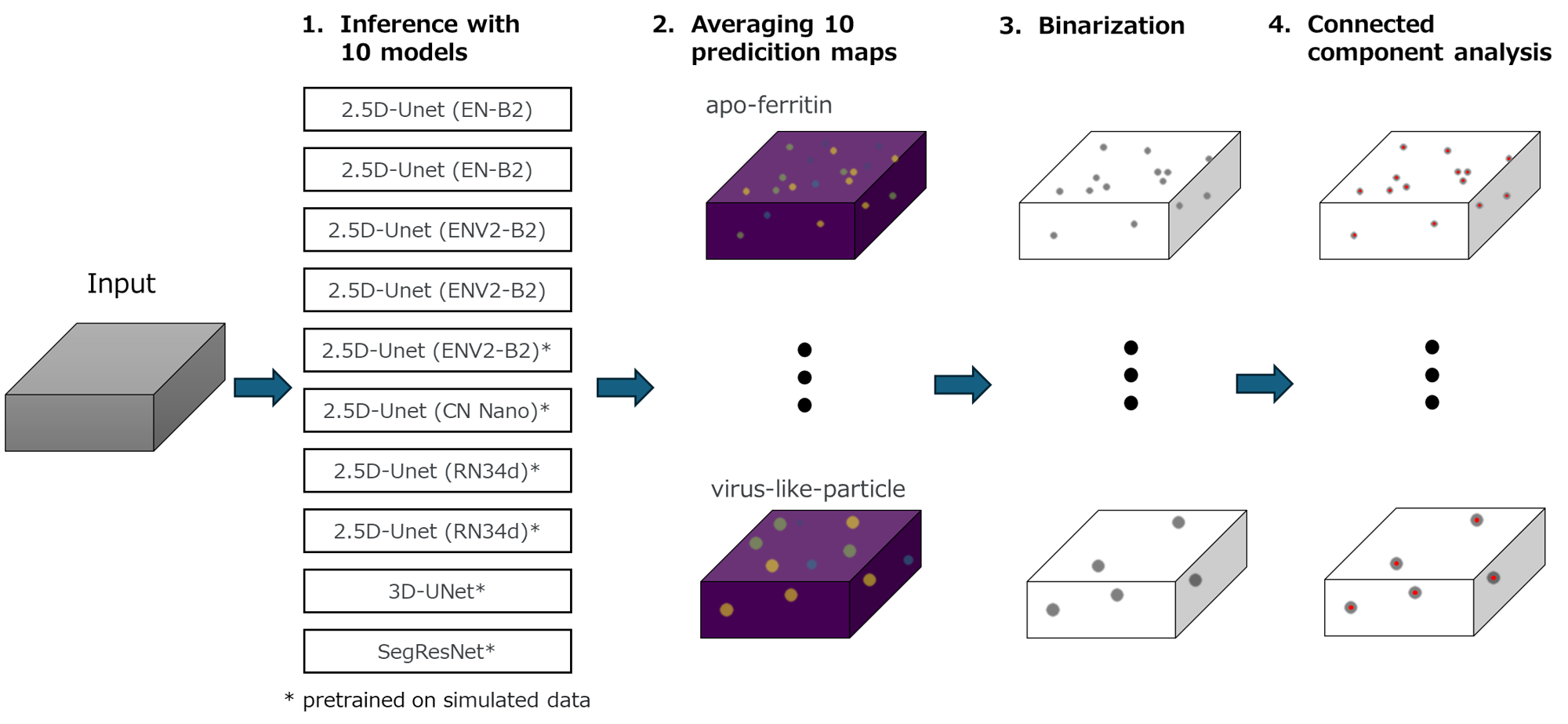\n\n# Models\nI utilized a 2.5D UNet based on [this notebook](https://www.kaggle.com/code/hengck23/3d-unet-using-2d-image-encoder), as well as MONAI’s 3D UNet and SegResNet. For the 2.5D UNet, timm's EfficientNet-B2, EfficientNetV2-B2, ConvNeXt-Nano, and ResNet34d were used as encoders. While the 3D UNet and SegResNet initially struggled to achieve good performance using only the training dataset, they reached a similar level of accuracy as the 2.5D UNet after pretraining on simulated data, which I will describe later.\nTo improve model diversity, I trained a total of 10 models with slight variations in pretraining strategies, data augmentation techniques, and other hyperparameters. For the final submission, I used models trained on the entire training dataset.\n\n# Training\n## Preprocessing\nAs a preprocessing step, I first removed outliers and then applied min-max normalization. The input volumes were cropped to a fixed size of 64×128×128.\n\n## Particle Mask\nFor the training labels, I generated binary masks centered around each particle’s location. Specifically, I set the region within radius × 0.5 to 1 and all other areas to 0. I created these masks separately for each particle.\n\n## Loss Function\nInitially, I experimented with BCE and Focal Loss, but these loss functions resulted in extremely slow convergence, likely due to the severe class imbalance. I then tried Dice Loss and Tversky Loss, which significantly accelerated training. However, these loss functions caused the model’s predictions to become overly binary, outputting only extreme values of 0 or 1. \nSince my pipeline ensembles prediction maps by averaging them and then applies a threshold for binarization, such prediction values were undesirable. To address this, I used FocalTversky++ loss as proposed in [this paper](https://arxiv.org/pdf/2111.00528). By using this loss, the model outputs prediction maps that reflect its confidence.\n\n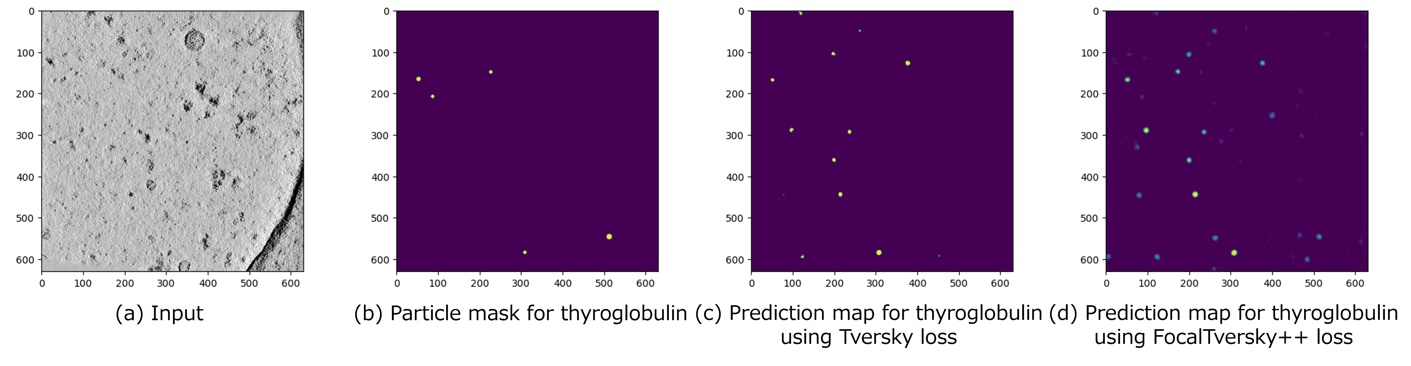\n\n## Pretraining with Simulated Data\nI generated my own simulated data using [polnet](https://github.com/anmartinezs/polnet) and used it to pretrain some of the models. To enhance the model’s ability to distinguish particles, I designed the simulated data to include particles with shapes similar to those of the target particles in this competition.\n\n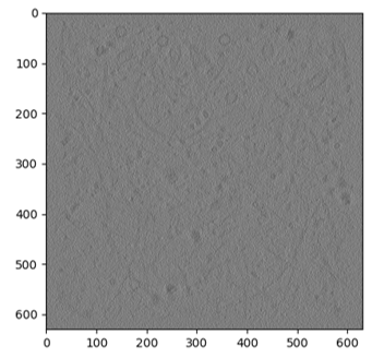\n\n# Inference\nFor inference, I used MONAI’s `sliding_window_inference` with an overlap ratio of 0.25. Since predictions near the edges of subvolumes tend to be less stable, I discarded the outermost 8% of predictions to improve reliability.\nI felt that one of the key challenges in this competition was achieving fast inference. To optimize speed, I first converted the models to TensorRT in a separate notebook before submission. During inference, I loaded the pre-converted TensorRT models and leveraged parallel processing with two T4 GPUs.\n\n# Post Processing\nOnce the ensembled prediction maps were obtained, I binarized them using particle-specific thresholds. These thresholds were initially estimated through cross-validation and later fine-tuned based on leaderboard.\nAfter binarization, I performed connected component analysis on the binary map and extracted the centroid of each connected component as the particle location.\n\n# What Did Not Work\n- Two-stage model\n- Use of tomogram data other than denoised\n\n# Code\n- https://github.com/uchiyama33/czii-6th-place\n- https://www.kaggle.com/code/tomoon33/czii-submission-6th-place", "3117038": "Congratulations!!! \nWould it be possible for you to share the single model score in the final solution?", "3117043": "Public LBs of the single model ranged from 0.757 to 0.766. \n(However, the thresholds in the single model were not fine-tuned, so the scores could be a bit higher if optimal thresholds were used.)", "3117180": "Interesting, thanks for sharing. \n\nWere you able to measure how much your CV/LB scores changed when using FocalTversky++ over Tversky?", "3117868": "Single model scores increased by about 0.02 for both CV and LB. While I can't provide exact values, the score improvement with ensembling was significantly larger when using FocalTversky++.", "3122272": "I’ve updated my solution code." }, "source": "meta" }