
First of all, I would like to sincerely thank the competition organizers, dataset providers, and the competitors for this interesting competition. It was very fun experimenting with different models, and I learned a lot in this competition. This is the solution for my 7th place submission.
\nMy approach utilized a 3D segmentation models with per class gaussian heatmap prediction. The models were first pre-trained on the simulated dataset (1fold, wbp as val) then fine tuned to the experimental dataset (4 fold). I trained all models using weighted BCE with very high pos_weight, to make the model generate more predictions. Heavy augmentations were performed during training, including Mixup, Cutmix, RandomFlip, Affine (only rotate in the xy plane, used in pre-training only), rot90(only in the xy plane), and other pixel-value augmentatons. The final submission consisted of an ensemble of three model soups (each combining four folds), applying 4x test-time augmentation (TTA) and a 4x sliding window approach.
\nTo reduce the pre-training time, I used the whole simulated dataset for training and used the wbp version of the experimental dataset for validation.
\nPreprocessing was minimal, involving percentile clipping (0.1–99.9%) and dataset-specific scaling factors:
\nI used a sliding window approach with a stride of 64, excluding the last window, to create 1x8x8=64 windows per experiment (0, 64, 128, …, 384, 448 for x and y, 0 for z), then randomly shifted the crop coordinates when generating the training data.
\nThe augmentations I used were:
\nI used 3 models in the final submission, 2 U-Net based models and 1 DeepLab based model. Among the two U-net based models, one has a backbone of ResNet50d and the other has a backbone of EfficientNetV2-M. The DeepLab based model has a backbone of ResNet50d. I tried training a model with an offset prediction head to improve the localization performance but it did not work in my case, so the final submission only uses a simple segmentation head. ModelEMA with a decay of 0.995 was for all models except model 207.
\n
Out of the 5 feature stages, only using the first 4 stages resulted in comparable or better performance, so some models (resnet50d) in the ensemble do that. I'm guessing it was because the high-resolution feature maps contained better information needed to locate the particles.
\nIn the final ensemble, backbones of [resnet50d, resnet50d, efficientnetv2-m] were used.
\nWhile it was not used in the final submission, DeepLabV3+ was also able to achieve relatively high scores, while only requiring half the inference time of the U-Net models. It may be able to create a better submission by using DeepLabV3+ and doing more ensembles.
\n| Model | \nBackbone | \nNo. skip connections | \nDecoder channels | \nInitial weights | \n
|---|---|---|---|---|
| Model 207 & 209 | \nResNet50d | \n4 | \n[128, 64, 32, 16] | \nra2_in1k | \n
| Model 248 & 249 | \nEfficientNetV2-M | \n5 | \n[512, 176, 80, 48, 24] | \nin21k_ft_in1k | \n
| Model | \nBackbone | \nNo. Highres features | \nNo. seg features | \nInitial weights | \n
|---|---|---|---|---|
| Model 258 & 265 | \nResNet50d | \n48 | \n256 | \nra2_in1k | \n
The loss function was a weighted BCE loss, where more weights were given to the \"hard\" particles, and regions where the target was positive. The formula for the loss function is given by
\n$$
\nL_{c, i} = -w_c \\left(p_c \\cdot y_{c, i} \\cdot \\log(t_{c, i}) + (1 - y_{c, i}) \\cdot \\log(1 - t_{c, i}) \\right)
\n$$
\n$$
\nLoss = \\frac{1}{5N} \\sum_{c=1}^{5} \\sum_{i=1}^{N} L_{c, i}
\n$$
where \\(L_{c, i}\\) is the loss for class \\(c\\) and pixel \\(i\\), \\(w_c\\) is the weight for class \\(c\\), \\(p_c\\) is the weight for the positive pixels in class \\(c\\), \\(y_{c, i}\\) is the prediction for class \\(c\\) and pixel \\(i\\), and \\(t_{c, i}\\) is the target for class \\(c\\) and pixel \\(i\\). \\(N\\) is the number of pixels in the image, and the sum is taken over all the pixels and classes.
\nThe class weights and the positive weights are shown below.
\nThe classes are in the order of [apo-ferritin, beta-galactosidase, ribosome, thyroglobulin, virus-like-particle].
| Model | \nClass Weights | \nPositive Weights | \n
|---|---|---|
| Model 207 | \n[1, 2, 1, 2, 1] | \n[28, 54, 36, 48, 24] | \n
| Model 209 | \n[1, 2, 1, 2, 1] | \n[54, 96, 24, 36, 36] | \n
| Model 248 | \n[1, 2, 1, 2, 1] × 5/7 | \n[24, 36, 36, 48, 20] | \n
| Model 249 | \n[1, 2, 1, 2, 1] × 5/7 | \n[54, 96, 36, 36, 36] | \n
| Model 258 | \n[1, 3, 2, 3, 1] | \n[42, 48, 72, 85, 54] | \n
| Model 265 | \n[1, 3, 2, 3, 1] | \n[54, 96, 24, 36, 36] | \n
Inference was performed on padded volumes of size (192, 128, 128). I created 81 windows out of the [184, 630, 630] tomogram with 64 stride on the x and y axis, resulting in 4x TTA. When combining the results to a single heatmap, averaging the logits was better than averaging the sigmoid-ed heatmaps.
\nTo reduce the edge artifact, I also applied a sloped weight function that goes down near the edge.
Flip augmentations were done as TTA. Depending on the number of models, 8x to 3x (normal, flipx, flipy) TTA was applied.
\nInitially I was using CCL + center of mass to determine the coordinates but I switched to using maxpool to detect the local maxima. To reduce noise, gaussian blur with kernel size 5 and sigma 1.0 was applied before the maxpool, and weighted box fusion with radius=0.5*particle_radius was applied after the local maxima detection. Using the maxpool method significantly improved the inference speed with minimal performance loss (~0.002 reduction), enabling me to do more TTAs and ensembles.
\nDue to the very high pos_weight, threshold of around 0.5 was enough to make the model predict many FPs. The final submission used thresholds of [0.3, 0.2, -0.2, -0.2, -0.2] in the logit space.
\nWhen ensembling the output of the different models, averaging the logits of the heatmaps were better compared to averaging the sigmoid-ed heatmap or applying WBF on the final predictions. 3 models with 4x Flip TTA, 4x Sliding Window seemed to be the best balance between TTA and ensemble.
\nBy making 3 submissions with only the targeted class
\nmat = np.array()\nTP, FP, FN = np.linalg.solve(mat, )\nAfter the total number of particles is obtained, TP, FP, FN can be calculated from 2 submissions. (by changing the bottom row of the coefficient matrix to 1, 0, 1 and the target to 0, -added_fp*more_fp_score, num_particles)
At first I was afraid to use this information to tune my model but the probed particle counts (TP + FN) matched the average counts stated in the paper (https://www.biorxiv.org/content/10.1101/2024.11.04.621686v1), so I assumed that the private test set had the same particle distribution as the public test set. I was trying to keep my submission count low in the first half of the competition to not overfit to the LB but after this I decided to trust the LB over my CV.
\n| Description | \nPublic Score | \nPrivate Score | \n
|---|---|---|
| Model 209 | \n0.77320 | \n0.76665 | \n
| Model 249 | \n0.77024 | \n0.76478 | \n
| Model 265 | \n0.76824 | \n0.76057 | \n
| Ensemble of the three | \n0.78351 | \n0.77708 | \n
First of all, I would like to sincerely thank the competition organizers, dataset providers, and the competitors for this interesting competition. It was very fun experimenting with different models, and I learned a lot in this competition. This is the solution for my 7th place submission.
\nMy approach utilized a 3D segmentation models with per class gaussian heatmap prediction. The models were first pre-trained on the simulated dataset (1fold, wbp as val) then fine tuned to the experimental dataset (4 fold). I trained all models using weighted BCE with very high pos_weight, to make the model generate more predictions. Heavy augmentations were performed during training, including Mixup, Cutmix, RandomFlip, Affine (only rotate in the xy plane, used in pre-training only), rot90(only in the xy plane), and other pixel-value augmentatons. The final submission consisted of an ensemble of three model soups (each combining four folds), applying 4x test-time augmentation (TTA) and a 4x sliding window approach.
\nTo reduce the pre-training time, I used the whole simulated dataset for training and used the wbp version of the experimental dataset for validation.
\nPreprocessing was minimal, involving percentile clipping (0.1–99.9%) and dataset-specific scaling factors:
\nI used a sliding window approach with a stride of 64, excluding the last window, to create 1x8x8=64 windows per experiment (0, 64, 128, …, 384, 448 for x and y, 0 for z), then randomly shifted the crop coordinates when generating the training data.
\nThe augmentations I used were:
\nI used 3 models in the final submission, 2 U-Net based models and 1 DeepLab based model. Among the two U-net based models, one has a backbone of ResNet50d and the other has a backbone of EfficientNetV2-M. The DeepLab based model has a backbone of ResNet50d. I tried training a model with an offset prediction head to improve the localization performance but it did not work in my case, so the final submission only uses a simple segmentation head. ModelEMA with a decay of 0.995 was for all models except model 207.
\n
Out of the 5 feature stages, only using the first 4 stages resulted in comparable or better performance, so some models (resnet50d) in the ensemble do that. I'm guessing it was because the high-resolution feature maps contained better information needed to locate the particles.
\nIn the final ensemble, backbones of [resnet50d, resnet50d, efficientnetv2-m] were used.
\nWhile it was not used in the final submission, DeepLabV3+ was also able to achieve relatively high scores, while only requiring half the inference time of the U-Net models. It may be able to create a better submission by using DeepLabV3+ and doing more ensembles.
\n| Model | \nBackbone | \nNo. skip connections | \nDecoder channels | \nInitial weights | \n
|---|---|---|---|---|
| Model 207 & 209 | \nResNet50d | \n4 | \n[128, 64, 32, 16] | \nra2_in1k | \n
| Model 248 & 249 | \nEfficientNetV2-M | \n5 | \n[512, 176, 80, 48, 24] | \nin21k_ft_in1k | \n
| Model | \nBackbone | \nNo. Highres features | \nNo. seg features | \nInitial weights | \n
|---|---|---|---|---|
| Model 258 & 265 | \nResNet50d | \n48 | \n256 | \nra2_in1k | \n
The loss function was a weighted BCE loss, where more weights were given to the \"hard\" particles, and regions where the target was positive. The formula for the loss function is given by
\n$$
\nL_{c, i} = -w_c \\left(p_c \\cdot y_{c, i} \\cdot \\log(t_{c, i}) + (1 - y_{c, i}) \\cdot \\log(1 - t_{c, i}) \\right)
\n$$
\n$$
\nLoss = \\frac{1}{5N} \\sum_{c=1}^{5} \\sum_{i=1}^{N} L_{c, i}
\n$$
where \\(L_{c, i}\\) is the loss for class \\(c\\) and pixel \\(i\\), \\(w_c\\) is the weight for class \\(c\\), \\(p_c\\) is the weight for the positive pixels in class \\(c\\), \\(y_{c, i}\\) is the prediction for class \\(c\\) and pixel \\(i\\), and \\(t_{c, i}\\) is the target for class \\(c\\) and pixel \\(i\\). \\(N\\) is the number of pixels in the image, and the sum is taken over all the pixels and classes.
\nThe class weights and the positive weights are shown below.
\nThe classes are in the order of [apo-ferritin, beta-galactosidase, ribosome, thyroglobulin, virus-like-particle].
| Model | \nClass Weights | \nPositive Weights | \n
|---|---|---|
| Model 207 | \n[1, 2, 1, 2, 1] | \n[28, 54, 36, 48, 24] | \n
| Model 209 | \n[1, 2, 1, 2, 1] | \n[54, 96, 24, 36, 36] | \n
| Model 248 | \n[1, 2, 1, 2, 1] × 5/7 | \n[24, 36, 36, 48, 20] | \n
| Model 249 | \n[1, 2, 1, 2, 1] × 5/7 | \n[54, 96, 36, 36, 36] | \n
| Model 258 | \n[1, 3, 2, 3, 1] | \n[42, 48, 72, 85, 54] | \n
| Model 265 | \n[1, 3, 2, 3, 1] | \n[54, 96, 24, 36, 36] | \n
Inference was performed on padded volumes of size (192, 128, 128). I created 81 windows out of the [184, 630, 630] tomogram with 64 stride on the x and y axis, resulting in 4x TTA. When combining the results to a single heatmap, averaging the logits was better than averaging the sigmoid-ed heatmaps.
\nTo reduce the edge artifact, I also applied a sloped weight function that goes down near the edge.
Flip augmentations were done as TTA. Depending on the number of models, 8x to 3x (normal, flipx, flipy) TTA was applied.
\nInitially I was using CCL + center of mass to determine the coordinates but I switched to using maxpool to detect the local maxima. To reduce noise, gaussian blur with kernel size 5 and sigma 1.0 was applied before the maxpool, and weighted box fusion with radius=0.5*particle_radius was applied after the local maxima detection. Using the maxpool method significantly improved the inference speed with minimal performance loss (~0.002 reduction), enabling me to do more TTAs and ensembles.
\nDue to the very high pos_weight, threshold of around 0.5 was enough to make the model predict many FPs. The final submission used thresholds of [0.3, 0.2, -0.2, -0.2, -0.2] in the logit space.
\nWhen ensembling the output of the different models, averaging the logits of the heatmaps were better compared to averaging the sigmoid-ed heatmap or applying WBF on the final predictions. 3 models with 4x Flip TTA, 4x Sliding Window seemed to be the best balance between TTA and ensemble.
\nBy making 3 submissions with only the targeted class
\nmat = np.array()\nTP, FP, FN = np.linalg.solve(mat, )\nAfter the total number of particles is obtained, TP, FP, FN can be calculated from 2 submissions. (by changing the bottom row of the coefficient matrix to 1, 0, 1 and the target to 0, -added_fp*more_fp_score, num_particles)
At first I was afraid to use this information to tune my model but the probed particle counts (TP + FN) matched the average counts stated in the paper (https://www.biorxiv.org/content/10.1101/2024.11.04.621686v1), so I assumed that the private test set had the same particle distribution as the public test set. I was trying to keep my submission count low in the first half of the competition to not overfit to the LB but after this I decided to trust the LB over my CV.
\n| Description | \nPublic Score | \nPrivate Score | \n
|---|---|---|
| Model 209 | \n0.77320 | \n0.76665 | \n
| Model 249 | \n0.77024 | \n0.76478 | \n
| Model 265 | \n0.76824 | \n0.76057 | \n
| Ensemble of the three | \n0.78351 | \n0.77708 | \n
Congratulations on your solo gold and the prize! That's a clever technique to probe the LB.
", "rawMarkdown": "Congratulations on your solo gold and the prize! That's a clever technique to probe the LB.", "votes": null }, { "id": "3128454", "postDate": "02/19/2025 15:16:36", "content": "It has been two weeks since the competition has ended, but I realized I was making an unbelievably stupid mistake of mixing up Experiment 265 (DeepLabV3+ architecture) with Experiment 256 (U-Net architecture). I am really sorry that I did not noticed this sooner. Also, the details of the loss function and the scores of the model has been added.
", "rawMarkdown": "It has been two weeks since the competition has ended, but I realized I was making an unbelievably stupid mistake of mixing up Experiment 265 (DeepLabV3+ architecture) with Experiment 256 (U-Net architecture). I am really sorry that I did not noticed this sooner. Also, the details of the loss function and the scores of the model has been added.", "votes": null }, { "id": "3129915", "postDate": "02/21/2025 05:57:17", "content": "Your writeup is impressively detailed—I truly appreciate the depth of insights you’ve shared.
", "rawMarkdown": "Your writeup is impressively detailed—I truly appreciate the depth of insights you’ve shared.", "votes": null }, { "id": "3365829", "postDate": "12/07/2025 11:49:30", "content": "Hi @kokikoba, Nice Writeup!! How were the class_weights and positive_weights were determined for each model?? Do you use any specific algorithm?
", "rawMarkdown": "Hi @kokikoba, Nice Writeup!! How were the class_weights and positive_weights were determined for each model?? Do you use any specific algorithm?", "votes": null } ], "comments": [ { "id": 3116832, "author_name": "snnclsr", "author_url": "", "post_date": "02/06/2025 11:02:26", "content": "Congratulations on your solo gold and the prize! That's a clever technique to probe the LB.
", "votes": null, "replies": [] }, { "id": 3128454, "author_name": "kokikoba", "author_url": "", "post_date": "02/19/2025 15:16:36", "content": "It has been two weeks since the competition has ended, but I realized I was making an unbelievably stupid mistake of mixing up Experiment 265 (DeepLabV3+ architecture) with Experiment 256 (U-Net architecture). I am really sorry that I did not noticed this sooner. Also, the details of the loss function and the scores of the model has been added.
", "votes": null, "replies": [] }, { "id": 3129915, "author_name": "linhanwang2", "author_url": "", "post_date": "02/21/2025 05:57:17", "content": "Your writeup is impressively detailed—I truly appreciate the depth of insights you’ve shared.
", "votes": null, "replies": [] }, { "id": 3365829, "author_name": "gowrishankarp", "author_url": "", "post_date": "12/07/2025 11:49:30", "content": "Hi @kokikoba, Nice Writeup!! How were the class_weights and positive_weights were determined for each model?? Do you use any specific algorithm?
", "votes": null, "replies": [] } ], "raw_markdown_by_id": { "3116629": "# 7th place solution\n\nFirst of all, I would like to sincerely thank the competition organizers, dataset providers, and the competitors for this interesting competition. It was very fun experimenting with different models, and I learned a lot in this competition. This is the solution for my 7th place submission.\n\n## Summary\n\nMy approach utilized a 3D segmentation models with per class gaussian heatmap prediction. The models were first pre-trained on the simulated dataset (1fold, wbp as val) then fine tuned to the experimental dataset (4 fold). I trained all models using weighted BCE with very high pos_weight, to make the model generate more predictions. Heavy augmentations were performed during training, including Mixup, Cutmix, RandomFlip, Affine (only rotate in the xy plane, used in pre-training only), rot90(only in the xy plane), and other pixel-value augmentatons. The final submission consisted of an ensemble of three model soups (each combining four folds), applying 4x test-time augmentation (TTA) and a 4x sliding window approach.\n\n## Pre-processing and data augmentations\n\nTo reduce the pre-training time, I used the whole simulated dataset for training and used the wbp version of the experimental dataset for validation.\n\nPreprocessing was minimal, involving percentile clipping (0.1–99.9%) and dataset-specific scaling factors:\n- Simulated: ×1.0\n- WBP: ×1e4\n- Denoised: ×1e5\n\nI used a sliding window approach with a stride of 64, excluding the last window, to create 1x8x8=64 windows per experiment (0, 64, 128, ..., 384, 448 for x and y, 0 for z), then randomly shifted the crop coordinates when generating the training data.\n\nThe augmentations I used were:\n- shift (up to 64 from the predetermined crop window)\n- cutmix\n- mixup\n- randomflip (all axis)\n- rot90 (only on xy plane)\n- affine (scale on every axis, rotate only on xy plane)\\*only when pre-training\n- contrast (0.7 ~ 1.5)\n- gamma (0.8 ~ 1.2)\n- gaussian noise (0 ~ 0.05)\\*only when fine tuning\n\n## Model architecture\n\nI used 3 models in the final submission, 2 U-Net based models and 1 DeepLab based model. Among the two U-net based models, one has a backbone of ResNet50d and the other has a backbone of EfficientNetV2-M. The DeepLab based model has a backbone of ResNet50d. I tried training a model with an offset prediction head to improve the localization performance but it did not work in my case, so the final submission only uses a simple segmentation head. ModelEMA with a decay of 0.995 was for all models except model 207.\n\n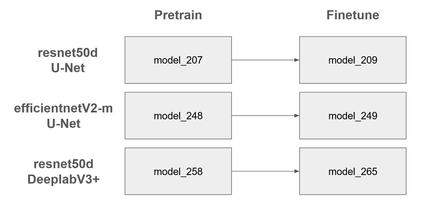\n\nOut of the 5 feature stages, only using the first 4 stages resulted in comparable or better performance, so some models (resnet50d) in the ensemble do that. I'm guessing it was because the high-resolution feature maps contained better information needed to locate the particles.\n\nIn the final ensemble, backbones of [resnet50d, resnet50d, efficientnetv2-m] were used.\n\nWhile it was not used in the final submission, DeepLabV3+ was also able to achieve relatively high scores, while only requiring half the inference time of the U-Net models. It may be able to create a better submission by using DeepLabV3+ and doing more ensembles.\n\n| Model | Backbone | No. skip connections | Decoder channels | Initial weights |\n|------------------|------------------|----------------------|--------------------------|-------------------|\n| Model 207 & 209 | ResNet50d | 4 | [128, 64, 32, 16] | ra2_in1k |\n| Model 248 & 249 | EfficientNetV2-M | 5 | [512, 176, 80, 48, 24] | in21k_ft_in1k |\n\n| Model | Backbone | No. Highres features | No. seg features | Initial weights |\n|-----------------|-----------|----------------------|------------------|-----------------|\n| Model 258 & 265 | ResNet50d | 48 | 256 | ra2_in1k |\n\n## Loss function\n\nThe loss function was a weighted BCE loss, where more weights were given to the \"hard\" particles, and regions where the target was positive. The formula for the loss function is given by\n\n$$\nL_{c, i} = -w_c \\left(p_c \\cdot y_{c, i} \\cdot \\log(t_{c, i}) + (1 - y_{c, i}) \\cdot \\log(1 - t_{c, i}) \\right)\n$$\n$$\nLoss = \\frac{1}{5N} \\sum_{c=1}^{5} \\sum_{i=1}^{N} L_{c, i}\n$$\n\nwhere \\\\(L_{c, i}\\\\) is the loss for class \\\\(c\\\\) and pixel \\\\(i\\\\), \\\\(w_c\\\\) is the weight for class \\\\(c\\\\), \\\\(p_c\\\\) is the weight for the positive pixels in class \\\\(c\\\\), \\\\(y_{c, i}\\\\) is the prediction for class \\\\(c\\\\) and pixel \\\\(i\\\\), and \\\\(t_{c, i}\\\\) is the target for class \\\\(c\\\\) and pixel \\\\(i\\\\). \\\\(N\\\\) is the number of pixels in the image, and the sum is taken over all the pixels and classes.\n\nThe class weights and the positive weights are shown below.\nThe classes are in the order of [apo-ferritin, beta-galactosidase, ribosome, thyroglobulin, virus-like-particle].\n| Model | Class Weights | Positive Weights |\n|------------|------------------------------|-------------------------|\n| Model 207 | [1, 2, 1, 2, 1] | [28, 54, 36, 48, 24] |\n| Model 209 | [1, 2, 1, 2, 1] | [54, 96, 24, 36, 36] |\n| Model 248 | [1, 2, 1, 2, 1] × 5/7 | [24, 36, 36, 48, 20] |\n| Model 249 | [1, 2, 1, 2, 1] × 5/7 | [54, 96, 36, 36, 36] |\n| Model 258 | [1, 3, 2, 3, 1] | [42, 48, 72, 85, 54] |\n| Model 265 | [1, 3, 2, 3, 1] | [54, 96, 24, 36, 36] |\n\n## Inference\n\nInference was performed on padded volumes of size (192, 128, 128). I created 81 windows out of the [184, 630, 630] tomogram with 64 stride on the x and y axis, resulting in 4x TTA. When combining the results to a single heatmap, averaging the logits was better than averaging the sigmoid-ed heatmaps.\nTo reduce the edge artifact, I also applied a sloped weight function that goes down near the edge.\n\nFlip augmentations were done as TTA. Depending on the number of models, 8x to 3x (normal, flipx, flipy) TTA was applied.\n\n## Postprocessing\n\nInitially I was using CCL + center of mass to determine the coordinates but I switched to using maxpool to detect the local maxima. To reduce noise, gaussian blur with kernel size 5 and sigma 1.0 was applied before the maxpool, and weighted box fusion with radius=0.5*particle_radius was applied after the local maxima detection. Using the maxpool method significantly improved the inference speed with minimal performance loss (~0.002 reduction), enabling me to do more TTAs and ensembles.\n\nDue to the very high pos_weight, threshold of around 0.5 was enough to make the model predict many FPs. The final submission used thresholds of [0.3, 0.2, -0.2, -0.2, -0.2] in the **logit space**.\n\n## Ensemble strategy\n\nWhen ensembling the output of the different models, averaging the logits of the heatmaps were better compared to averaging the sigmoid-ed heatmap or applying WBF on the final predictions. 3 models with 4x Flip TTA, 4x Sliding Window seemed to be the best balance between TTA and ensemble.\n\n\n## Probing the LB\n\nBy making 3 submissions with only the targeted class\n- Normal\n- Added FP (like appending (0, 0, 0) * 20 to every prediction)\n- Doubled prediction\nit is able to calculate the number of TP, FP, FNs by solving the system of equations:\n```\nmat = np.array([\n \t[17*(original_score - 1), original_score, 16*original_score],\n \t[17*(more_fp_score - 1), more_fp_score, 16*more_fp_score],\n \t[18*double_pred_score - 17, 2*double_pred_score, 16*double_pred_score]\n\t])\nTP, FP, FN = np.linalg.solve(mat, [0, -added_fp*more_fp_score, 0])\n```\n\nAfter the total number of particles is obtained, TP, FP, FN can be calculated from 2 submissions. (by changing the bottom row of the coefficient matrix to `1, 0, 1` and the target to `0, -added_fp*more_fp_score, num_particles`)\n\n\nAt first I was afraid to use this information to tune my model but the probed particle counts (TP + FN) matched the average counts stated in the paper (https://www.biorxiv.org/content/10.1101/2024.11.04.621686v1), so I assumed that the private test set had the same particle distribution as the public test set. I was trying to keep my submission count low in the first half of the competition to not overfit to the LB but after this I decided to trust the LB over my CV.\n\n\n## Scores\n| Description | Public Score | Private Score |\n|---------------------------------|--------------|---------------|\n| Model 209 | 0.77320 | 0.76665 |\n| Model 249 | 0.77024 | 0.76478 |\n| Model 265 | 0.76824 | 0.76057 |\n|Ensemble of the three| 0.78351 | 0.77708 |", "3116832": "Congratulations on your solo gold and the prize! That's a clever technique to probe the LB.", "3128454": "It has been two weeks since the competition has ended, but I realized I was making an unbelievably stupid mistake of mixing up Experiment 265 (DeepLabV3+ architecture) with Experiment 256 (U-Net architecture). I am really sorry that I did not noticed this sooner. Also, the details of the loss function and the scores of the model has been added.", "3129915": "Your writeup is impressively detailed—I truly appreciate the depth of insights you’ve shared.", "3365829": "Hi @kokikoba, Nice Writeup!! How were the class_weights and positive_weights were determined for each model?? Do you use any specific algorithm?" }, "source": "meta" }