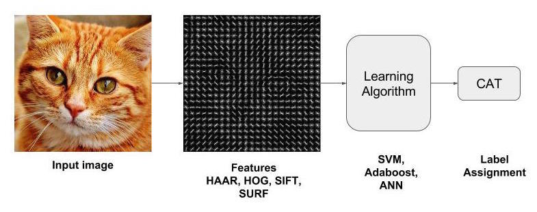
\n"], "metadata": {"_uuid": "b82449f2853efd1db7c5ee5051872711dd945c79", "_cell_guid": "c59f8e06-be43-4a78-bd09-1b43dbeccab2"}, "cell_type": "markdown"}, {"source": [" ## Introduction\n", "\n", "Image classification involves assigning a label/s to an image based on its features. the traditional steps (process pipeline) carried out by an image classification system are:\n", "\n", "
Preprocessing: highly dependant on the image/ how its captured also the features to be extracted, a very common preprocessing operation is normalisation, i.e. subtract mean and devide by standard deviation i.e $\\frac {x-\\bar{x}}{\\sigma}$. Another is gamma correction
\n", "
Feature Extraction : the design of good features to extract used to play the most critical role in the design of the image classifier. That seems to have changed with the emmergance of deep learning
\n", "
Learning Model Selection: the design of different classifiers with tools such as [logistic regression](https://en.wikipedia.org/wiki/Logistic_regression), [Support Vector Machines SVM](https://en.wikipedia.org/wiki/Support_vector_machine), and [Adaboost](https://en.wikipedia.org/wiki/AdaBoost).
\n", "
Label Assignment
\n", ""], "metadata": {"_uuid": "998fddf18e40317fc0ff6fc3f3dd5876535e160f", "_cell_guid": "c7c497f5-e8bd-48ae-889f-dbda01102ac3"}, "cell_type": "markdown"}, {"source": ["Below is a visualisation of the classification process pipline\n", "Image classification pipeline [source](http://www.learnopencv.com/image-recognition-and-object-detection-part1/)"], "metadata": {"_uuid": "55dcda41ba677d504619985ad64959ac09af0315", "_cell_guid": "a458e44f-8a16-4fb8-a6f2-52c5e9905ab3"}, "cell_type": "markdown"}, {"source": ["\n", "the main categories of features i.e. \n", "
\n", "
Low Level Features such as \n", "
GIST
SIFT
HOG descriptors.
\n", "
Meduim level Features such as\n", "
\n", "
The Bag-of-Features (BoF) model
\n", "
The Spatial-Pyramid-Matching (SPM) model
\n", "
the Oriented Pyramid Matching (OPM) model. [TODO add refrence]
\n", "
\n", "
\n", "
High-Level Features such as \n", "
\n", "
Object Bank
\n", "
\n", "
\n", "\n", "
"], "metadata": {"_uuid": "c4e8d06b6f3e44151b72838e54f58501813c240b", "_cell_guid": "03caecde-b71a-43b2-b24d-94316ea56b2d"}, "cell_type": "markdown"}, {"source": ["### Python Libraries\n", "[OpenCV](http://opencv.org/) is an open source library used mainly by Computer Vision practitionors. I used it extensively in the past with `C++` and briefly with `Python`. so this kernel is really an opportunity for me to trasfer those skills\n", "I will also be using [scikit image](http://scikit-image.org/)\n", "also leargist"], "metadata": {"_uuid": "9f4e30501d4330eda6fd15f131b6b55cbd632f6b", "_cell_guid": "b20826ee-43f5-45c3-8659-2c33d77e2451"}, "cell_type": "markdown"}, {"source": ["import pandas as pd\n", "import numpy as np\n", "import bson\n", "import numpy as np\n", "\n", "\n", "import matplotlib.pyplot as plt\n", "import seaborn as sns\n", "from matplotlib import cm\n", "import matplotlib.gridspec as gridspec\n", "import cv2 #opencv library \n", "from skimage import data, io, filters,exposure, feature #essential when extracting features\n", "from skimage.transform import (hough_line, hough_line_peaks,\n", " probabilistic_hough_line)\n", "from sklearn.decomposition import PCA #princble component analysis\n", "# import keras\n", "# from keras.preprocessing import image as image_utils\n", "from IPython.display import Javascript\n", "# try:\n", "# import leargist\n", "# except:\n", "# !conda install leargist -y"], "execution_count": null, "metadata": {"collapsed": true, "_uuid": "69d2f60ea815912daec71effa42a470c6074a258", "_cell_guid": "e4247924-275c-40c5-b1e2-d99c3628ff5c"}, "cell_type": "code", "outputs": []}, {"source": ["path = '../input/'\n", "!ls \"$path\""], "execution_count": null, "metadata": {"collapsed": true, "_uuid": "f4819fe071e35294188487b0ca4581773b3943ab", "_cell_guid": "bc577e0e-1ebf-4895-a22c-9fb85d2c7460"}, "cell_type": "code", "outputs": []}, {"source": ["### Read Files"], "metadata": {"_uuid": "b098aa074fdefad0304399f1b48c454ecc0e6ef8", "_cell_guid": "fd9ab510-a956-484e-95af-a900c777ea45"}, "cell_type": "markdown"}, {"source": ["#### Read bson file and convert to pandas DataFrame"], "metadata": {"_uuid": "56ea1ba90258d79ca7254fff2dde4a385321f6d4", "_cell_guid": "17fc803e-5350-4b20-bcbc-be348738d6c5"}, "cell_type": "markdown"}, {"source": ["with open('{}{}'.format(path,'train_example.bson'),'rb') as b:\n", " df = pd.DataFrame(bson.decode_all(b.read()))\n", "#read and convert to opencv image\n", "df['imgs'] = df['imgs'].apply(lambda rec: cv2.imdecode(\n", " np.fromstring(rec[0]['picture'], np.uint8), cv2.IMREAD_COLOR))\n", "#change index to catergory id\n", "df.set_index('category_id',inplace=True)\n", "# Combine images and categries\n", "df.head()"], "execution_count": null, "metadata": {"collapsed": true, "_uuid": "4fa168dcd1047f38951ab529e2fb3d5bc633043b", "_cell_guid": "3dd561e5-409f-46d2-8159-fab560c5c36c"}, "cell_type": "code", "outputs": []}, {"source": ["df.info()"], "execution_count": null, "metadata": {"collapsed": true, "_uuid": "d62ebe1d207d7820639fc04c8fc160df106dcdc7", "_cell_guid": "ab5e7f4e-9501-4675-9e5d-f942982feba3"}, "cell_type": "code", "outputs": []}, {"source": ["## Image Classification\n", "### Pre-processing\n", "#### Normalisation"], "metadata": {"_uuid": "11d2a300d25bc18bed3511f0cec5941573bc89f8", "_cell_guid": "d44c128d-c343-4926-a6d6-0f31c0ba1b9e"}, "cell_type": "markdown"}, {"source": ["Convert to gray scale: this will generate the intensity part of the image using the equation I =0.299R+0.587G+0.114B. If I recall correctly, the weights in the equation are derived from understaning how each color receptor works in the human visual cotex see [here](https://en.wikipedia.org/wiki/Grayscale) to understand the concept"], "metadata": {"_uuid": "16506b7f50a1a71933e52ccf0972d1bc3774a59f", "_cell_guid": "c4bdae45-c9b9-4d0f-8589-b6fec4799ad0"}, "cell_type": "markdown"}, {"source": ["#read the image\n", "image = df.iloc[80,-1]\n", "gray = .299 * image[...,0] + .587 * image[...,1]+ .114* image[...,2]"], "execution_count": null, "metadata": {"collapsed": true, "_uuid": "01eced37f3cf502e423cea4dffbef2ffdd360da9", "_cell_guid": "5cb787ce-9163-45de-91fa-a2dc05a8db04"}, "cell_type": "code", "outputs": []}, {"source": ["Apply $\\frac {x-\\bar{x}}{\\sigma}$. The mean is subtracted so that the image histogram is centralised around zero and the division by sigma performs the actual normalisation"], "metadata": {"_uuid": "727af4cd19be02672e45db186c6a6e78025d9e10", "_cell_guid": "61e693e1-6f21-48e8-8578-a1dcbca7ba7d"}, "cell_type": "markdown"}, {"source": ["normed_gray = (gray - gray[:].mean())/gray[:].std()"], "execution_count": null, "metadata": {"collapsed": true, "_uuid": "bae0217e55a0ddcd78e4138efea3029e5e71101e", "_cell_guid": "556a9073-7d73-4094-9245-1455b16b2cfa"}, "cell_type": "code", "outputs": []}, {"source": ["#### PCA-whitening\n"], "metadata": {"_uuid": "65b18266a0d4d5c016310087d7a54e1c16332121", "_cell_guid": "ed198f33-2205-4e50-b7c7-91d498747750"}, "cell_type": "markdown"}, {"source": ["gray -= gray[:].mean()# zero-center\n", "covariance_matrix = np.dot(gray.transpose(), gray) / gray.shape[0] \n", "# compute the SVD factorization of the data covariance matrix\n", "U,S,V = np.linalg.svd(covariance_matrix) \n", "rotation = np.dot(gray, U) # decorrelate the data\n", "whitened_gray = rotation / np.sqrt(S+1e-6)\n"], "execution_count": null, "metadata": {"collapsed": true, "_uuid": "ced57186b1b5dae14c476dfb3431f1d174967bd7", "_cell_guid": "57c7ab81-96b6-4385-aafa-48d0e4eec3a7"}, "cell_type": "code", "outputs": []}, {"source": ["#plot both\n", "sns.set_style('white')\n", "fig, axs = plt.subplots(2,2, figsize=(8,8))\n", "axs = axs.flatten()\n", "imgs = [image ,gray,normed_gray,whitened_gray]\n", "titles = ['Original','GrayScale','Normalised','PCA-Whitened']\n", "for i, ax in enumerate(axs):\n", " if i<3:\n", " ax.imshow(imgs[i],aspect='auto',interpolation='nearest')\n", " else:\n", " ax.imshow(imgs[i],aspect='auto',interpolation='nearest',cmap='gray')\n", " ax.set_title(titles[i])\n", " ax.axis('off')\n", "plt.tight_layout()\n", "plt.show()"], "execution_count": null, "metadata": {"collapsed": true, "_uuid": "c712e932c49ff2c264753aeb21b13b8e45e60951", "_cell_guid": "c66e9b69-c103-4156-98b9-ae38816ad27d"}, "cell_type": "code", "outputs": []}, {"source": ["## Feature Extraction\n", "### Canny Edge Detection\n", "The Process of Canny edge detection algorithm can be broken down to 5 different steps: \n", "\n", "\n", "
Apply Gaussian filter to smooth the image in order to remove the noise
\n", "
Find the intensity gradients of the image
\n", "
Apply non-maximum suppression to get rid of spurious response to edge detection
\n", "
Apply double threshold to determine potential edges
\n", "
Track edge by hysteresis: Finalize the detection of edges by suppressing all the other edges that are weak and not connected to strong edges.
\n", "\n", " \n", "Source: [https://en.wikipedia.org/wiki/Canny_edge_detector](https://en.wikipedia.org/wiki/Canny_edge_detector)"], "metadata": {"_uuid": "f5e2659b36f33ea516c574ac97c00d71b8518a64", "_cell_guid": "6f9aea11-e406-4a8f-8cf3-380249bb785e"}, "cell_type": "markdown"}, {"source": ["#%%javascript\n", "#// $('#help').height(20);"], "execution_count": null, "metadata": {"collapsed": true, "_uuid": "fd8ae7c4ca99263ec1c975373356aa6533351a32", "_cell_guid": "af23794e-d243-47ce-ac29-5a6558ab5755"}, "cell_type": "code", "outputs": []}, {"source": ["edges = feature.canny(normed_gray,low_threshold =2,sigma=.5)\n", "# help(feature.canny)\n", "# #create refrence to style output\n", "# Javascript('this.element.attr(\"id\", \"help\")')"], "execution_count": null, "metadata": {"collapsed": true, "_uuid": "d021661c6d0390e8cbf77d5e3646d1fee485395a", "_cell_guid": "0426ef97-ffc9-4af0-afa5-8d5a4e64671c"}, "cell_type": "code", "outputs": []}, {"source": ["### Hough Transform\n", "The purpose of the technique is to find imperfect instances of objects within a certain class of shapes by a voting procedure. This voting procedure is carried out in a parameter space, from which object candidates are obtained as local maxima in a so-called accumulator space that is explicitly constructed by the algorithm for computing the Hough transform.\n", "\n", "The classical Hough transform was concerned with the identification of lines in the image, but later the Hough transform has been extended to identifying positions of arbitrary shapes, most commonly circles or ellipses. \n", "