{"cells":[{"metadata":{},"cell_type":"markdown","source":"# <center>Cassava Leaf Disease Classification</center>\n# ![image](https://i.ytimg.com/vi/VGCHcgmZu24/maxresdefault.jpg)"},{"metadata":{},"cell_type":"markdown","source":"In this Notebook,  I am going to build a model from scratch using keras framework and analyse how augmentation, different input sizes, image proprocessing techniques impact the accuracy of the model. To start with this, I have chosen an artchitecture mentioned in paper titled **\"A predictive machine learning application in agriculture: Cassava disease detection and classification with imbalanced dataset using convolutional neural networks\"** published in 2020. This architecture with hyperparameter tuning and preprocessing was able to achieve 93% accuracy in Cassava 2019 CVPR challenge.\n\n## Contents:\n\n- [About competition](#s1)\n- [Importing necessary Libraries](#s2)\n- [Previous Experimentation Results](#s9)\n- [Dataset Description](#se3)\n - [Class Distribution](#ss31)\n - [Sample Images](#ss32)\n- [Necessary Functions](#s11)\n - [Random Cropping](#ss111)\n - [CLAHE](#sss112)\n- [Train-Valid Split](#s4)\n- [Model Architecture](#s5)\n- [Training](#s6)\n- [Model Visualization](#s7)\n- [Prediction](#s8)\n- [Next Steps](#s10)"},{"metadata":{},"cell_type":"markdown","source":"<a id=\"s1\"> </a>\n## About Competition\n\nCassava, or Manihot esculenta, belongs to the family Euphorbiaceae and is cultivated in tropical and subtropical regions for its edible starchy tuberous root, which is commonly dried into a powder and named tapioca.\n\nAs the second-largest provider of carbohydrates in Africa, cassava is a key food security crop grown by smallholder farmers because it can withstand harsh conditions. At least 80% of household farms in Sub-Saharan Africa grow this starchy root, but viral diseases are major sources of poor yields. With the help of data science, it may be possible to identify common diseases so they can be treated.\n\nExisting methods of disease detection require farmers to solicit the help of government-funded agricultural experts to visually inspect and diagnose the plants. This suffers from being labor-intensive, low-supply and costly. As an added challenge, effective solutions for farmers must perform well under significant constraints, since African farmers may only have access to mobile-quality cameras with low-bandwidth.\n\nIn this competition, we introduce a dataset of 21,367 labeled images collected during a regular survey in Uganda. Most images were crowdsourced from farmers taking photos of their gardens, and annotated by experts at the National Crops Resources Research Institute (NaCRRI) in collaboration with the AI lab at Makerere University, Kampala. This is in a format that most realistically represents what farmers would need to diagnose in real life.\n\n### HEALTH BENEFITS\n\nTapioca has been associated with some health benefits, such as **healthy weight gain, increased red blood cell count, improved digestion, preventing diabetes, protecting bone mineral density, preventing Alzheimer’s disease and maintaining fluid balance within the body.**\n\n### EVALUATION\n**$$Accuracy=\\frac{TP + TN}{TP + FP + TN + FN}$$**\n\nwhere,  \n - TP: True Positive\n - FP: False Positive\n - TN: True Negative\n - FN: False Negative"},{"metadata":{},"cell_type":"markdown","source":"<a id ='s2'></a>\n## Importing Necessary Libraries"},{"metadata":{"_uuid":"8f2839f25d086af736a60e9eeb907d3b93b6e0e5","_cell_guid":"b1076dfc-b9ad-4769-8c92-a6c4dae69d19","trusted":true},"cell_type":"code","source":"#numpy - for necessary matric operation\nimport numpy as np\n\n#pandas to work with dataframes\nimport pandas as pd\n\n#keras - Model Building\nfrom keras.preprocessing.image import ImageDataGenerator\nfrom keras.layers import Conv2D,BatchNormalization,MaxPool2D,Dense,Flatten,Dropout\nfrom keras.models import Sequential,load_model,Model\nfrom keras.callbacks import ModelCheckpoint,EarlyStopping,ReduceLROnPlateau\nfrom keras.optimizers import Adam\n\n#cv2 - for image operations\nimport cv2\n#reading disease names from provided json file\nimport json\n\nimport time\n\n#visualizations\nimport plotly.graph_objs as go\nimport matplotlib.pyplot as plt\nimport seaborn as sns\nfrom plotly.subplots import make_subplots\nfrom sklearn.manifold import TSNE\nfrom tqdm.notebook import tqdm\n\n#oversampling technique\nfrom imblearn.over_sampling import SMOTE\n\n#train-test split\nfrom sklearn.model_selection import train_test_split","execution_count":null,"outputs":[]},{"metadata":{},"cell_type":"markdown","source":"<a id='s9'></a>\n## Previous Experimentation Results"},{"metadata":{"trusted":true},"cell_type":"code","source":"fig = go.Figure()\nt1 = go.Bar(x=['Without Augmentation','With Augmentation','Augmentation and CLAHE'],y=[0.687,0.683,0.332],text = [0.687,0.683,0.332],textposition='auto')\nfig.add_trace(t1)\nfig.update_xaxes(title_text=\"Experimentations\")\nfig.update_yaxes(title_text=\"Score\")\nfig.update_layout(title='Public Score')\nfig.show()","execution_count":null,"outputs":[]},{"metadata":{},"cell_type":"markdown","source":"<a id='s3'></a>\n## Dataset Description"},{"metadata":{"_uuid":"d629ff2d2480ee46fbb7e2d37f6b5fab8052498a","_cell_guid":"79c7e3d0-c299-4dcb-8224-4455121ee9b0","trusted":true},"cell_type":"code","source":"#reading training data\ntrain_df = pd.read_csv('../input/cassava-leaf-disease-classification/train.csv')\n#maping the class labels mentioned in json file wiht its respective disease name\ndisease_names = open('../input/cassava-leaf-disease-classification/label_num_to_disease_map.json')\ndisease_names = json.load(disease_names)\n\n#parse through every label value and identify the disease name based on label number from json file\ntrain_df['disease_name'] = train_df['label'].apply(lambda x: disease_names[str(x)])\n#visualize the top five rows from table\ntrain_df.head()","execution_count":null,"outputs":[]},{"metadata":{},"cell_type":"markdown","source":"<a id='ss31'></a>\n### Class Labels Distribution"},{"metadata":{"trusted":true},"cell_type":"code","source":"fig = make_subplots(rows=1, cols=2,\n            specs=[[{\"type\": \"xy\"}, {\"type\": \"domain\"}]],)\n# value_counts: to count number of images in each class with respect to disease_name column\n# Bar plot \nt1 = go.Bar(x=train_df['disease_name'].value_counts().index, \n            y=train_df['disease_name'].value_counts().values,\n            text=train_df['disease_name'].value_counts().values,\n            textposition='auto',name='Count',\n           marker_color='indianred')\n#Pie chart with labels and counts\nt2 = go.Pie(labels=train_df['disease_name'].value_counts().index,\n           values=train_df['disease_name'].value_counts().values,\n           hole=0.3)\nfig.add_trace(t1,row=1, col=1)\nfig.add_trace(t2,row=1, col=2)\nfig.update_layout(title='Distribution of Class Labels')\nfig.show()","execution_count":null,"outputs":[]},{"metadata":{},"cell_type":"markdown","source":"<a id=\"s32\"></a>\n### Sample Images from each class"},{"metadata":{"trusted":true},"cell_type":"code","source":"#random seed is used to replicate the same images in every run\nnp.random.seed(2020)\n#plotting 5 random samples for each class with image name and disease name as title\nfor class_name in train_df['disease_name'].unique():\n    plt.figure(figsize=(20,50))\n    for idx,img_name in enumerate(np.random.choice(train_df[train_df['disease_name'] == class_name]['image_id'].values,\n                                                   size=5,replace=False)):\n        plt.subplot(1,5,idx+1)\n        #reading the image and converting BGR color space to RGB\n        img = cv2.cvtColor(cv2.imread('../input/cassava-leaf-disease-classification/train_images/'+img_name), cv2.COLOR_BGR2RGB)\n        plt.imshow(img)\n        plt.axis('off')\n        plt.title(r\"$\\bf{\"+class_name + \"}$\"+'\\n'+img_name )\n    plt.show()","execution_count":null,"outputs":[]},{"metadata":{},"cell_type":"markdown","source":"<a id='ss11'></a>\n### Necessary Functions"},{"metadata":{},"cell_type":"markdown","source":"<a id='sss111'></a>\n### Random Cropping"},{"metadata":{"trusted":true},"cell_type":"code","source":"def random_crop(img, random_crop_size):\n    # Note: image_data_format is 'channel_last'\n    assert img.shape[2] == 3\n    height, width = img.shape[0], img.shape[1]\n    dy, dx = random_crop_size\n    x = np.random.randint(0, width - dx + 1)\n    y = np.random.randint(0, height - dy + 1)\n    return img[y:(y+dy), x:(x+dx), :]\n\n\ndef crop_generator(batches, crop_length):\n    \"\"\"Take as input a Keras ImageGen (Iterator) and generate random\n    crops from the image batches generated by the original iterator.\n    \"\"\"\n    while True:\n        batch_x, batch_y = next(batches)\n        batch_crops = np.zeros((batch_x.shape[0], crop_length, crop_length, 3))\n        for i in range(batch_x.shape[0]):\n            batch_crops[i] = random_crop(batch_x[i], (crop_length, crop_length))\n        yield batch_crops, batch_y","execution_count":null,"outputs":[]},{"metadata":{},"cell_type":"markdown","source":"<a id='sss112'></a>\n### CLAHE: Pre-processing\n\n**Contrast Limited AHE:**\n\nAdaptive histogram equalization (AHE) is a computer image processing technique used to improve contrast in images. It differs from ordinary histogram equalization in the respect that the adaptive method computes several histograms, each corresponding to a distinct section of the image, and uses them to redistribute the lightness values of the image. It is therefore suitable for improving the local contrast and enhancing the definitions of edges in each region of an image.\n\n**Contrast limited AHE** limits the contrast amplification to reduce amplified noise. It does so by distributing that part of the histogram that exceeds the clip limit equally across all histograms."},{"metadata":{"trusted":true},"cell_type":"code","source":"def clahe_preprocessing(img):\n    planes = cv2.split(img.astype(np.uint8))\n    clahe = cv2.createCLAHE(clipLimit=2.0, tileGridSize=(8, 8))\n    for j in range(len(planes)):\n        planes[j] = clahe.apply(planes[j])\n    return cv2.merge(planes)","execution_count":null,"outputs":[]},{"metadata":{},"cell_type":"markdown","source":"<a id='s4'></a>\n## Train-Valid Split"},{"metadata":{},"cell_type":"markdown","source":"Splitting 20% of the training data for validating the model"},{"metadata":{"trusted":true},"cell_type":"code","source":"VALIDATION_SPLIT_PERCENT = 0.2\nTRAINING_IMGS_DIR = '../input/cassava-leaf-disease-classification/train_images/'\nIMAGE_ID_COL_NAME = 'image_id'\nLABEL_ID_COL_NAME = 'disease_name' #or label\nTARGET_SIZE = 512\nBATCH_SIZE = 8\nCLASS_MODE = 'sparse'","execution_count":null,"outputs":[]},{"metadata":{},"cell_type":"markdown","source":"### SMOTE: Synthetic Minority Oversampling Technique\n\nReference: https://www.analyticsvidhya.com/blog/2020/10/overcoming-class-imbalance-using-smote-techniques/\n\nSMOTE is an oversampling technique where the synthetic samples are generated for the minority class. This algorithm helps to overcome the overfitting problem posed by random oversampling. It focuses on the feature space to generate new instances with the help of interpolation between the positive instances that lie together.\n\nAt first the total no. of oversampling observations, N is set up. Generally, it is selected such that the binary class distribution is 1:1. But that could be tuned down based on need. Then the iteration starts by first selecting a positive class instance at random. Next, the KNN’s (by default 5) for that instance is obtained. At last, N of these K instances is chosen to interpolate new synthetic instances. To do that, using any distance metric the difference in distance between the feature vector and its neighbors is calculated. Now, this difference is multiplied by any random value in (0,1] and is added to the previous feature vector. This is pictorially represented below:\n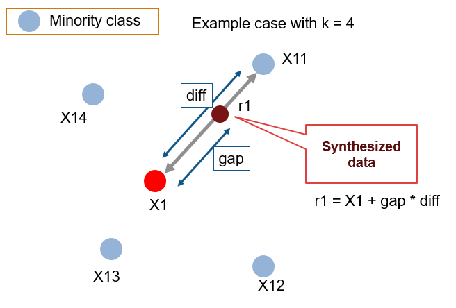![image](https://editor.analyticsvidhya.com/uploads/77417image1.png)"},{"metadata":{"trusted":true},"cell_type":"code","source":"#smt = SMOTE()\n#read all the images in train data and store it in a variable(train_x,train_y) and apply smot as below\n#since it involves a huge size of storing it in a variable throwing a memory error- So i am holding SMOTE processing for now and do the Hypoer Parameter tuning\n#train_x_smt,train_y_smt = smt.fit_resample(train_x.reshape(len(train_x),-1),train_y)","execution_count":null,"outputs":[]},{"metadata":{},"cell_type":"markdown","source":"### Load Train and Valid images"},{"metadata":{"trusted":true},"cell_type":"code","source":"#generate images and split 20% for validation\ntrain_data = ImageDataGenerator(validation_split=VALIDATION_SPLIT_PERCENT,\n                                horizontal_flip=True,\n                                vertical_flip=True,\n                                shear_range=0.1,\n                                rescale=1,\n                                zoom_range=0.2,\n                                width_shift_range=0.1,\n                                height_shift_range=0.1)\ntrain_gen = train_data.flow_from_dataframe(train_df,\n                                           directory= TRAINING_IMGS_DIR,\n                                           subset=\"training\",\n                                           x_col= IMAGE_ID_COL_NAME,\n                                           y_col= LABEL_ID_COL_NAME,\n                                          target_size=(TARGET_SIZE,TARGET_SIZE),\n                                           batch_size=BATCH_SIZE,\n                                           class_mode=CLASS_MODE)\ntrain_images = crop_generator(train_gen,TARGET_SIZE)\nvalid_data = ImageDataGenerator(validation_split=VALIDATION_SPLIT_PERCENT)\nvalid_gen = valid_data.flow_from_dataframe(train_df,\n                                           directory= TRAINING_IMGS_DIR,\n                                           subset=\"validation\",\n                                           x_col=IMAGE_ID_COL_NAME,\n                                           y_col= LABEL_ID_COL_NAME,\n                                          target_size=(TARGET_SIZE,TARGET_SIZE),\n                                           batch_size=BATCH_SIZE,\n                                           class_mode=CLASS_MODE)","execution_count":null,"outputs":[]},{"metadata":{"trusted":true},"cell_type":"code","source":"fig = go.Figure()\nt1 = go.Bar(name='Train',x=np.unique(train_gen.labels,return_counts=True)[0],y=np.unique(train_gen.labels,return_counts=True)[1],\n           text=np.unique(train_gen.labels,return_counts=True)[1],textposition='auto')\nt2 = go.Bar(name='Valid',x=np.unique(valid_gen.labels,return_counts=True)[0],y=np.unique(valid_gen.labels,return_counts=True)[1],\n           text=np.unique(valid_gen.labels,return_counts=True)[1],textposition='auto')\nfig.add_trace(t1)\nfig.add_trace(t2)\n#x-axis and y axis title\nfig.update_xaxes(title_text=\"Class Labels\")\nfig.update_yaxes(title_text=\"Number of Images\")\nfig.update_layout(title='Train and Valid Split')\nfig.show()\n\n#Pie Chart\nfig = make_subplots(rows=1, cols=2,subplot_titles=['Train Data', 'Valid Data'],\n            specs=[[{\"type\": \"domain\"}, {\"type\": \"domain\"}]],)\n\n#Pie chart with labels and counts\nt1 = go.Pie(labels=np.unique(train_gen.labels,return_counts=True)[0],\n           values=np.unique(train_gen.labels,return_counts=True)[1],\n           hole=0.3)\nt2 = go.Pie(labels=np.unique(valid_gen.labels,return_counts=True)[0],\n           values=np.unique(valid_gen.labels,return_counts=True)[1],\n           hole=0.3)\nfig.add_trace(t1,row=1, col=1)\nfig.add_trace(t2,row=1, col=2)\nfig.update_layout(title='Distribution in Train and Valid Split')\nfig.show()","execution_count":null,"outputs":[]},{"metadata":{},"cell_type":"markdown","source":"<a id='s5'></a>\n## Model Architecture       "},{"metadata":{"trusted":true},"cell_type":"code","source":"def model_architecture(IMG_SIZE):\n    #arrange the model in sequential manner\n    model = Sequential()\n    #First Convolutional Layer\n    model.add(Conv2D(32,(5,5),activation='relu',input_shape=(IMG_SIZE,IMG_SIZE,3)))\n    model.add(BatchNormalization())\n    model.add(MaxPool2D((3,3)))\n    #Second Convolutional Layer\n    model.add(Conv2D(64,(3,3),activation='relu'))\n    model.add(BatchNormalization())\n    model.add(MaxPool2D((3,3)))\n    #Third Convolutional Layer\n    model.add(Conv2D(128,(3,3),activation='relu'))\n    model.add(BatchNormalization())\n    model.add(MaxPool2D((3,3)))\n    #flatten the architecture\n    model.add(Flatten())\n    \n    #First Dense Layer with 1% dropout ratio\n    model.add(Dense(512,activation='relu'))\n    model.add(Dropout(0.1))\n    #Second Dense Layer with 1% dropout ratio\n    model.add(Dense(1024,activation='relu'))\n    model.add(Dropout(0.1))\n    #Third Dense Layer with 1% dropout ratio\n    model.add(Dense(1024,activation='relu'))\n    model.add(Dropout(0.1))\n    #Fourth Dense Layer with 1% dropout ratio\n    model.add(Dense(256,activation='relu'))\n    model.add(Dropout(0.1))\n    #Output layer\n    model.add(Dense(5,activation='softmax'))\n    model.summary()\n    \n    #compile the model with Adam optimizer\n    model.compile(optimizer = Adam(lr = 0.001),\n                  loss = \"sparse_categorical_crossentropy\",\n                  metrics = [\"acc\"])\n    return model","execution_count":null,"outputs":[]},{"metadata":{"trusted":true},"cell_type":"code","source":"STEPS_PER_EPOCH = len(train_gen) / BATCH_SIZE\nVALIDATION_STEPS = len(valid_gen) / BATCH_SIZE\nEPOCHS = 100\nMODEL_NAME = './cvpr_2019_model_with_augmentation_512_100_epochs.h5'","execution_count":null,"outputs":[]},{"metadata":{"trusted":true},"cell_type":"code","source":"model = model_architecture(TARGET_SIZE)","execution_count":null,"outputs":[]},{"metadata":{"trusted":true},"cell_type":"code","source":"#callbacks\nmodel_save = ModelCheckpoint(MODEL_NAME, \n                             save_best_only = True, \n                             save_weights_only = True,\n                             monitor = 'val_loss', \n                             mode = 'min', verbose = 1)\nearly_stop = EarlyStopping(monitor = 'val_loss', min_delta = 0.001, \n                           patience = 5, mode = 'min', verbose = 1,\n                           restore_best_weights = True)\nreduce_lr = ReduceLROnPlateau(monitor = 'val_loss', factor = 0.3, \n                              patience = 2, min_delta = 0.001, \n                              mode = 'min', verbose = 1)","execution_count":null,"outputs":[]},{"metadata":{},"cell_type":"markdown","source":"<a id='s6'></a>\n## Training"},{"metadata":{"trusted":true},"cell_type":"code","source":"history = model.fit(\n    train_images,\n    steps_per_epoch = STEPS_PER_EPOCH,\n    epochs = EPOCHS,\n    validation_data = valid_gen,\n    validation_steps = VALIDATION_STEPS,\n    callbacks = [model_save, early_stop, reduce_lr]\n)","execution_count":null,"outputs":[]},{"metadata":{"trusted":true},"cell_type":"code","source":"acc = history.history['acc']\nval_acc = history.history['val_acc']\nloss = history.history['loss']\nval_loss = history.history['val_loss']\n\nepochs = [e for e in range(1, len(acc) + 1)]\n\nfig = make_subplots(rows=1, cols=2,subplot_titles=['Accuracy', 'Loss'],\n            specs=[[{\"type\": \"xy\"}, {\"type\": \"xy\"}]],)\n\nt1 = go.Scatter(x=epochs,y=acc,name='Training',mode='markers+lines',line={'color': 'blue'})\nt2 = go.Scatter(x=epochs,y=val_acc,name='Validation',mode='markers+lines',line={'dash': 'dash','color': 'red'})\n\nt3 = go.Scatter(x=epochs,y=loss,name='Training',mode='markers+lines',line={'color': 'blue'},showlegend=False)\nt4 = go.Scatter(x=epochs,y=val_loss,name='Validation',mode='markers+lines',line={'dash': 'dash','color': 'red'},showlegend=False)\n\nfig.add_trace(t1,row=1, col=1)\nfig.add_trace(t2,row=1, col=1)\n\nfig.add_trace(t3,row=1, col=2)\nfig.add_trace(t4,row=1, col=2)\n\nfig.update_layout(title='Training History')\nfig.show()","execution_count":null,"outputs":[]},{"metadata":{},"cell_type":"markdown","source":"<a id='s7'></a>\n## Model Visualization\n\nI read one interesting kernel recently, which explains how to visualize the trained model.   \n\nhttps://www.kaggle.com/harininarasimhan/why-not-to-trust-public-lb-visualization\n\nThank you **Harini Narasimhan** for sharing this kernel\n"},{"metadata":{"trusted":true},"cell_type":"code","source":"model.load_weights(MODEL_NAME)","execution_count":null,"outputs":[]},{"metadata":{},"cell_type":"markdown","source":"### Train Model Visualization"},{"metadata":{"trusted":true},"cell_type":"code","source":"intermediater_layer_model = Model(inputs=model.inputs, outputs = model.get_layer('dense_3').output)\nintermediate_output = intermediater_layer_model.predict(train_gen,verbose=1,batch_size=BATCH_SIZE)\nintermediate_output.shape","execution_count":null,"outputs":[]},{"metadata":{"trusted":true},"cell_type":"code","source":"st_time = time.time()\nt_sne = TSNE(random_state=2020)\nt_sne_tr = t_sne.fit_transform(intermediate_output)\nprint('TNSE done; Time take {} seconds'.format(time.time()-st_time))\n##T-SNE df\ntsne_tr = pd.DataFrame()\nfor idx in range(t_sne_tr.shape[1]):\n    tsne_tr['t_sne'+str(idx+1)] = t_sne_tr[:,idx]\ntsne_tr['label'] = np.array(train_gen.labels).astype(int)\ntsne_tr['disease_name'] = tsne_tr['label'].apply(lambda x: disease_names[str(x)])\nfig = go.Figure()\ncolors = ['rgb(243, 247, 15)','rgb(13, 160, 200)','rgb(190, 81, 249)','rgb(248, 104, 73)','rgb(0,255,0)']\nfor idx,dn in enumerate(tsne_tr['disease_name'].unique()):\n    df = tsne_tr[tsne_tr['disease_name'] == dn]\n    fig.add_trace(go.Scatter(x=df['t_sne1'],y=df['t_sne2'],mode='markers',marker_color = colors[idx],name=dn))\nfig.update_layout(title='Trained model performance')\nfig.update_xaxes(title_text=\"TSNE_1\")\nfig.update_yaxes(title_text=\"TSNE_2\")\nfig.show()","execution_count":null,"outputs":[]},{"metadata":{},"cell_type":"markdown","source":"### Valid Model Visualization"},{"metadata":{"trusted":true},"cell_type":"code","source":"intermediater_layer_model = Model(inputs=model.inputs, outputs = model.get_layer('dense_3').output)\nintermediate_output = intermediater_layer_model.predict(valid_gen,verbose=1,batch_size=BATCH_SIZE)","execution_count":null,"outputs":[]},{"metadata":{"trusted":true},"cell_type":"code","source":"st_time = time.time()\nt_sne = TSNE(random_state=2020)\nt_sne_va = t_sne.fit_transform(intermediate_output)\nprint('TNSE done; Time take {} seconds'.format(time.time()-st_time))\n##T-SNE df\ntsne_va = pd.DataFrame()\nfor idx in range(t_sne_va.shape[1]):\n    tsne_va['t_sne'+str(idx+1)] = t_sne_va[:,idx]\ntsne_va['label'] = np.array(valid_gen.labels).astype(int)\ntsne_va['disease_name'] = tsne_va['label'].apply(lambda x: disease_names[str(x)])\nfig = go.Figure()\ncolors = ['rgb(243, 247, 15)','rgb(13, 160, 200)','rgb(190, 81, 249)','rgb(248, 104, 73)','rgb(0,255,0)']\nfor idx,dn in enumerate(tsne_va['disease_name'].unique()):\n    df = tsne_va[tsne_va['disease_name'] == dn]\n    fig.add_trace(go.Scatter(x=df['t_sne1'],y=df['t_sne2'],mode='markers',marker_color = colors[idx],name=dn))\nfig.update_layout(title='Validated model performance')\nfig.update_xaxes(title_text=\"TSNE_1\")\nfig.update_yaxes(title_text=\"TSNE_2\")\nfig.show()","execution_count":null,"outputs":[]},{"metadata":{},"cell_type":"markdown","source":"<a id='s8'></a>\n## Prediction"},{"metadata":{"trusted":true},"cell_type":"code","source":"ss = pd.read_csv(\"../input/cassava-leaf-disease-classification/sample_submission.csv\")\npreds = []\n\nfor image_id in ss.image_id:\n    image = cv2.cvtColor(cv2.imread('../input/cassava-leaf-disease-classification/test_images/'+image_id),cv2.COLOR_BGR2RGB)\n    image = cv2.resize(image,(TARGET_SIZE,TARGET_SIZE))\n    image = np.expand_dims(image, axis = 0)\n    preds.append(np.argmax(model.predict(image)))\n\nss['label'] = preds\nss.to_csv('submission.csv', index = False)","execution_count":null,"outputs":[]},{"metadata":{"trusted":true},"cell_type":"markdown","source":"<a id='s10'></a>\n## Next Steps"},{"metadata":{"trusted":true},"cell_type":"markdown","source":"- SMOTE to address imbalance nature of image - On Hold\n- Hyper Parameter Tuning"},{"metadata":{},"cell_type":"markdown","source":"**Do Upvote !!!**"}],"metadata":{"kernelspec":{"language":"python","display_name":"Python 3","name":"python3"},"language_info":{"pygments_lexer":"ipython3","nbconvert_exporter":"python","version":"3.6.4","file_extension":".py","codemirror_mode":{"name":"ipython","version":3},"name":"python","mimetype":"text/x-python"}},"nbformat":4,"nbformat_minor":4}