{"metadata":{"kernelspec":{"language":"python","display_name":"Python 3","name":"python3"},"language_info":{"name":"python","version":"3.7.6","mimetype":"text/x-python","codemirror_mode":{"name":"ipython","version":3},"pygments_lexer":"ipython3","nbconvert_exporter":"python","file_extension":".py"},"kaggle":{"accelerator":"none","dataSources":[{"sourceId":13836,"databundleVersionId":1718836,"sourceType":"competition"}],"dockerImageVersionId":30042,"isInternetEnabled":true,"language":"python","sourceType":"notebook","isGpuEnabled":false}},"nbformat_minor":4,"nbformat":4,"cells":[{"cell_type":"markdown","source":"","metadata":{}},{"cell_type":"markdown","source":" About Competiton
\n\nAs the second-largest provider of carbohydrates in Africa, cassava is a key food security crop grown by smallholder farmers because it can withstand harsh conditions. At least 80% of household farms in Sub-Saharan Africa grow this starchy root, but viral diseases are major sources of poor yields. With the help of data science, it may be possible to identify common diseases so they can be treated.\n\nExisting methods of disease detection require farmers to solicit the help of government-funded agricultural experts to visually inspect and diagnose the plants. This suffers from being labor-intensive, low-supply and costly. As an added challenge, effective solutions for farmers must perform well under significant constraints, since African farmers may only have access to mobile-quality cameras with low-bandwidth.\n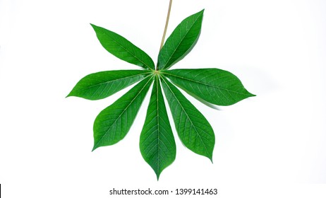\n\n fig.1: Cassava Leaf\n \n \n \n### Task\nclassify each cassava image into four disease categories or a fifth category indicating a healthy leaf.\n\nclasses Name\n\n0. CBB (Cassava Bactrial Blight)\n1. CBSD (Cassava Brown Streak Disease)\n2. CGM (Cassava Green Mottle)\n3. CMD (Cassava Mosaic Disease)\n4. Healthy ","metadata":{}},{"cell_type":"markdown","source":"\nWork Flow
\n\n\n\n\n\n","metadata":{}},{"cell_type":"markdown","source":" Import Library
\nA programming library is simply code that is already written, already tested, and ready for you to link to and use. Why are libraries useful? These can greatly reduce the amount of time to write code.","metadata":{}},{"cell_type":"code","source":"import os\nimport pandas as pd\nimport numpy as np\nimport seaborn as sb\nfrom PIL import Image\nimport matplotlib.pyplot as plt\nimport json\nimport cv2\nfrom skimage import io, img_as_ubyte\nfrom skimage import util\nfrom sklearn.model_selection import train_test_split\nfrom keras.preprocessing.image import ImageDataGenerator\nfrom skimage.filters import threshold_multiotsu\nfrom skimage import io, img_as_ubyte\n","metadata":{"trusted":true},"execution_count":null,"outputs":[]},{"cell_type":"markdown","source":" Define Working Directory
\n\nIn computing, the working directory of a process is a directory of a hierarchical file system.","metadata":{}},{"cell_type":"code","source":"main_dir = '../input/cassava-leaf-disease-classification/'\nos.listdir(main_dir) \ntrain_img_path = '../input/cassava-leaf-disease-classification/train_images'","metadata":{"trusted":true},"execution_count":null,"outputs":[]},{"cell_type":"markdown","source":" Data visualization
\n\nData visualization is the practice of translating information into a visual context, such as a map or graph, to make data easier for the human brain to understand and pull insights from. The main goal of data visualization is to make it easier to identify patterns, trends and outliers in large data sets.","metadata":{}},{"cell_type":"markdown","source":"## Load CSV file\n\nCSV is a simple file format used to store tabular data, such as a spreadsheet or database","metadata":{}},{"cell_type":"code","source":"dataframe = pd.read_csv(main_dir+'train.csv')\n\nimgs_id = dataframe['image_id'].values\nimgs_label = dataframe['label'].values\nprint('Head of the CSV file \\n\\n',dataframe.head())\nprint('\\n Lenght of the image label : ',len(dataframe['label']))\nprint('\\n length of the image id :', len(dataframe['image_id']))\n","metadata":{"trusted":true},"execution_count":null,"outputs":[]},{"cell_type":"markdown","source":"## Import JSON File\n\nJavaScript Object Notation (JSON) is a standard text-based format for representing structured data .","metadata":{}},{"cell_type":"code","source":"js = open(main_dir + 'label_num_to_disease_map.json')\nreal_classes = json.load(js)\nreal_classes = {int(k):v for k,v in real_classes.items()}\ndataframe['class_name'] = dataframe.label.map(real_classes)\n\nprint(dataframe['class_name']) \n \n ","metadata":{"trusted":true},"execution_count":null,"outputs":[]},{"cell_type":"markdown","source":"## Image With Class Label\n\nUsing matplotlib images and their labels are displayed.","metadata":{}},{"cell_type":"code","source":"def show_image(img_ids, img_classes):\n plt.figure(figsize=(16, 12))\n \n for i, (img_id, img_class) in enumerate(zip(img_ids, img_classes)):\n plt.subplot(3, 3, i + 1)\n image = cv2.imread(os.path.join(main_dir, \"train_images\", img_id))\n# image = cv2.cvtColor(image, cv2.COLOR_BGR2RGB)\n image = image[:, :, ::-1]\n \n plt.imshow(image)\n plt.title(f\"Class: {img_class}\", fontsize=12)\n plt.axis(\"off\")\n \n plt.show()","metadata":{"trusted":true},"execution_count":null,"outputs":[]},{"cell_type":"code","source":"\nnew_df = dataframe.sample(9)\nimg_ids = new_df[\"image_id\"].values\nlabels = new_df[\"class_name\"].values\n\nshow_image(img_ids, labels)","metadata":{"trusted":true},"execution_count":null,"outputs":[]},{"cell_type":"markdown","source":"## Histogram\nA histogram is a graphical display of data using bars of different heights.\n\nIts make easiler to understand , how much images have every classes and can compare it.","metadata":{}},{"cell_type":"code","source":"def hist_graph(y):\n fig = plt.figure()\n ax = fig.add_subplot(111)\n ax.hist(y, color='blue', linewidth =3)\n plt.title('Amount of images in five classes', fontsize=15)\n plt.xticks(np.arange(5))\n plt.xlabel('Classes')\n plt.ylabel('No. of images') \n plt.show() \n \n\nprint(real_classes) \nhist_graph( dataframe['label'])\n\n ","metadata":{"trusted":true},"execution_count":null,"outputs":[]},{"cell_type":"markdown","source":"Image Segmentation
\n\n\nSegmentation of an image is in practice for the classification of image pixel . Segmentation techniques are used to isolate the desired object from the image in order to perform analysis of the object.","metadata":{}},{"cell_type":"markdown","source":"### Forground Extraction (GrabCut)\n\nGrabCut is an image segmentation method based on graph cuts. Starting with a user-specified bounding box around the object to be segmented, the algorithm estimates the color distribution of the target object and that of the background using a Gaussian mixture model.","metadata":{}},{"cell_type":"code","source":"\n \ndef fg_extrac(img_ids, img_classes):\n plt.figure(figsize=(20, 16))\n for i, (img_id, img_class) in enumerate(zip(img_ids, img_classes)):\n plt.subplot(2,2, i + 1)\n \n src = train_img_path+'/'+img_id\n img= io.imread(src)\n mask = np.zeros(img.shape[:2],np.uint8)\n bgdModel = np.zeros((1,65),np.float64)\n fgdModel = np.zeros((1,65),np.float64)\n rect = (10,10,750,550)#left,top,right,bottom\n cv2.grabCut(img,mask,rect,bgdModel,fgdModel,5,cv2.GC_INIT_WITH_RECT)\n mask2 = np.where((mask==2)|(mask==0),0,1).astype('uint8')\n img = img*mask2[:,:,np.newaxis] \n \n plt.imshow(img)\n plt.title(f\"Class: {img_class}\", fontsize=12)\n plt.show()","metadata":{"trusted":true},"execution_count":null,"outputs":[]},{"cell_type":"code","source":"df = dataframe[10:14]\nimg_ids = df[\"image_id\"].values\nlabels = df[\"class_name\"].values\nfg_extrac(img_ids, labels)","metadata":{"trusted":true},"execution_count":null,"outputs":[]},{"cell_type":"markdown","source":"### GRAY\n\nGray is a cool, neutral, and balanced color. The color gray is an emotionless, moody color that is typically associated with meanings of dull, dirty, and dingy, as well as formal, conservative, and sophisticated.","metadata":{}},{"cell_type":"code","source":"\n \ndef gray(img_ids, img_classes):\n plt.figure(figsize=(16, 12))\n \n for i, (img_id, img_class) in enumerate(zip(img_ids, img_classes)):\n plt.subplot(2, 3, i + 1)\n src = train_img_path+'/'+img_id\n img= io.imread(src)\n# gray = cv2.cvtColor(img, cv2.COLOR_BGR2GRAY)\n gray = img[:, :, ::-1]\n \n plt.imshow(gray)\n plt.title(f\"Class: {img_class}\", fontsize=12)\n plt.axis(\"off\")\n \n plt.show()\n\n ","metadata":{"trusted":true},"execution_count":null,"outputs":[]},{"cell_type":"code","source":"df = dataframe.sample(6)\nimg_ids = df[\"image_id\"].values\nlabels = df[\"class_name\"].values\n\ngray(img_ids, labels)","metadata":{"trusted":true},"execution_count":null,"outputs":[]},{"cell_type":"markdown","source":"### Morphological transformations\n\nMorphological transformations are some simple opera ons based on the image shape. It is\nnormally performed on binary images. It needs two inputs, one is our original image, second\none is called structuring element or kernel which decides the nature of opera on.\n","metadata":{}},{"cell_type":"code","source":" \ndef thresh(img_ids, img_classes):\n plt.figure(figsize=(20, 16))\n \n for i, (img_id, img_class) in enumerate(zip(img_ids, img_classes)):\n plt.subplot(2, 3, i + 1)\n src = train_img_path+'/'+img_id\n img= io.imread(src)\n kernel = np.ones((5,5),np.uint8)\n morpo = cv2.morphologyEx(img, cv2.MORPH_GRADIENT, kernel)\n plt.imshow(morpo)\n plt.title(f\"Class: {img_class}\", fontsize=12)\n plt.axis(\"off\")\n \n plt.show()\n\n \n","metadata":{"trusted":true},"execution_count":null,"outputs":[]},{"cell_type":"code","source":"thresh(img_ids, labels)","metadata":{"trusted":true},"execution_count":null,"outputs":[]},{"cell_type":"markdown","source":"### Skimage\n\nScikit-image, or skimage, is an open source Python package designed for image preprocessing.\n","metadata":{}},{"cell_type":"code","source":"\n\n \ndef color_manipulation(img_ids, img_classes):\n plt.figure(figsize=(16, 12))\n \n for i, (img_id, img_class) in enumerate(zip(img_ids, img_classes)):\n plt.subplot(2,3, i + 1)\n src = train_img_path+'/'+img_id\n img= io.imread(src)\n inverted_img = util.invert(img)\n plt.imshow(inverted_img)\n plt.title(f\"Class: {img_class}\", fontsize=12)\n plt.axis(\"off\")\n \n plt.show()\n\n ","metadata":{"trusted":true},"execution_count":null,"outputs":[]},{"cell_type":"code","source":"df = dataframe[2010:2016]\nimg_ids = df[\"image_id\"].values\nlabels = df[\"class_name\"].values\n\ncolor_manipulation(img_ids, labels)","metadata":{"trusted":true},"execution_count":null,"outputs":[]},{"cell_type":"markdown","source":"### Thresold\n\nImage thresholding is a simple form of image segmentation. It is a way to create a binary image from a grayscale or full-color image. This is typically done in order to separate \"object\" or foreground pixels from background pixels to aid in image processing.\n","metadata":{}},{"cell_type":"code","source":" \n\n \ndef thresold(img_ids, img_classes):\n plt.figure(figsize=(16, 12))\n \n for i, (img_id, img_class) in enumerate(zip(img_ids, img_classes)):\n plt.subplot(2,3, i + 1)\n src = train_img_path+'/'+img_id\n img= io.imread(src)\n thresh = cv2.threshold(img,170,255,cv2.THRESH_BINARY)[1]\n \n plt.imshow(thresh)\n plt.title(f\"Class: {img_class}\", fontsize=12)\n plt.axis(\"off\")\n \n plt.show()\n\n ","metadata":{"trusted":true},"execution_count":null,"outputs":[]},{"cell_type":"code","source":"\nthresold(img_ids, labels)","metadata":{"trusted":true},"execution_count":null,"outputs":[]},{"cell_type":"markdown","source":"## Color Intensity","metadata":{}},{"cell_type":"code","source":"def color_intensity(img_ids, img_classes):\n plt.figure(figsize=(16, 12))\n \n for i, (img_id, img_class) in enumerate(zip(img_ids, img_classes)):\n plt.subplot(2,3, i + 1)\n src = train_img_path+'/'+img_id\n img= io.imread(src)\n hist = plt.hist(img.ravel(), bins = 256, color = 'orange', )\n hist = plt.hist(img[:, :, 0].ravel(), bins = 256, color = 'red', alpha = 0.5)\n hist = plt.hist(img[:, :, 1].ravel(), bins = 256, color = 'Green', alpha = 0.5)\n hist = plt.hist(img[:, :, 2].ravel(), bins = 256, color = 'Blue', alpha = 0.5)\n hist = plt.xlabel('Intensity Value')\n hist = plt.ylabel('Count')\n hist = plt.legend(['Total', 'Red Channel', 'Green Channel', 'Blue Channel'])\n \n plt.title(f\"Class: {img_class}\", fontsize=12)\n \n plt.show()","metadata":{"trusted":true},"execution_count":null,"outputs":[]},{"cell_type":"code","source":"color_intensity(img_ids, labels)","metadata":{"trusted":true},"execution_count":null,"outputs":[]},{"cell_type":"markdown","source":"# Image data split between train and validation\n","metadata":{}},{"cell_type":"code","source":"\n\ntrain,val = train_test_split(dataframe, test_size = 0.3, random_state = 42, stratify = dataframe['class_name'])\n","metadata":{"trusted":true},"execution_count":null,"outputs":[]},{"cell_type":"markdown","source":" Data Agumentation
\nData augmentation in data analysis are techniques used to increase the amount of data by adding slightly modified copies of already existing data or newly created synthetic data from existing data. It acts as a regularizer and helps reduce overfitting when training a machine learning model.\n\n\n\n Fig.2: After agumentation image","metadata":{}},{"cell_type":"code","source":"\nimg_row= 400\nimg_col=400\n\ntrain_datagen = ImageDataGenerator(rescale = 1/255.0,\n rotation_range = 40,\n width_shift_range = 0.4,\n height_shift_range = 0.4,\n shear_range = 0.4,\n zoom_range = 0.1,\n horizontal_flip = True,\n vertical_flip = True,\n featurewise_center = True,\n samplewise_center = True, \n featurewise_std_normalization= True,\n samplewise_std_normalization = True, \n fill_mode = 'nearest')\n\nvalidation_datagen = ImageDataGenerator(rescale=1.0/255)\n\ntrain_generator = train_datagen.flow_from_dataframe(train,\n directory = train_img_path,\n x_col = 'image_id',\n y_col = 'class_name',\n target_size = (img_row,img_col),\n color_mode = 'rgb',\n class_mode = 'categorical',\n interpolation = 'nearest',\n shuffle = True,\n batch_size = 64, \n )\n\n\nvalidation_generator = validation_datagen.flow_from_dataframe(val,\n directory = train_img_path,\n x_col = 'image_id',\n y_col = 'class_name',\n target_size = (img_row,img_col),\n color_mode = 'rgb',\n class_mode = 'categorical',\n interpolation = 'nearest',\n shuffle = True,\n batch_size = 64, \n )\n","metadata":{"trusted":true},"execution_count":null,"outputs":[]},{"cell_type":"markdown","source":"## Train and validatiion classes indices","metadata":{}},{"cell_type":"code","source":"print('train classes Name and indices: \\n',train_generator.class_indices)\nprint('validation classes Name and indices: \\n',validation_generator.class_indices)","metadata":{"trusted":true},"execution_count":null,"outputs":[]},{"cell_type":"markdown","source":"## Cassava leaf after agumentation ","metadata":{}},{"cell_type":"code","source":"for image, label in validation_generator:\n plt.figure(figsize= (16,12))\n print(image.shape)\n for i in range(0,6):\n plt.subplot(2,3,1+i)\n plt.imshow(image[i], cmap ='gray') \n plt.show()\n break","metadata":{"trusted":true},"execution_count":null,"outputs":[]},{"cell_type":"markdown","source":"# Model development using CNN\n[Cassava model & evalution](https://www.kaggle.com/code/jitshil143/keras-model)","metadata":{}},{"cell_type":"markdown","source":"# Reference\n\nhttps://www.wikipedia.org/\nhttps://stackoverflow.com/\nhttps://matplotlib.org/\nhttps://pandas.pydata.org/\nhttps://www.python.org/doc/","metadata":{}},{"cell_type":"markdown","source":"# Thank you for reading \n","metadata":{}}]}