{"cells":[{"metadata":{},"cell_type":"markdown","source":"\n DataScience Tackling Bird Vocalizations !\n
\n
\n\n Introduction to Audio Processing\n
\n\n---\n\n\n \n \n\n\n\n\n---\n\n
\nWhat it's all about?\n
\n
\nOne thing that I love about DataScience is its beauty of Versatility or the Diversity of Problem set we deal with. \n\nSome Days before I was working on a [CVD](https://www.kaggle.com/rahulgulia/datascience-tackling-heart-diseases/) problem and Now I'm here, trying my best to extract the soul / insight from [Cornell Birdcall Identification](https://www.kaggle.com/c/birdsong-recognition/overview) Dataset provided by Cornell Lab of Ornithology where :\n\n> * We'll identify a Wide variety of Bird Vocalizations in Soundscape Recordings.\n\nBut Catch is We have Weak Label i.e. :\n> * There might be anthropogenic sounds (e.g., airplane overflights) or other bird and non-bird (e.g., chipmunk) calls in the background, with a particular labeled bird species in the foreground\n\n---\n\nIn this Kernel, Right Now, We'll just try to extract some initial insights from the Dataset.\nObviously, Work is in process. I'll keep of updating this Kernel as the time flies to cover-up new findings :)\n\nIn the fast paced world, We are so busy in our life that we forget that we're not alone on this planet.
\nThis Competition gives an opportunity to connect back to some of those such sounds of beautiful creatures that will make us feel connected to our nature world. \n
\nSo, Relax and Let's get it started!\n\n\n**This gonna be a long kernel. So, Hey! Looking for a guide :) ?**\n
\n 1. Introduction
\n 1.1. What our Host says
\n 1.2. Directory Structure
\n 2. A Closer look to our Directories
\n 2.1. Exploring Training Meta Data
\n 2.1.1. Missing Values
\n 2.1.2. Feature : ebird_code (Target)
\n 2.1.3. Feature : recordist
\n 2.1.4. Feature : location, country, latitute, longitute
\n 2.1.5. Feature : date
\n 2.2. Exploring Training Data (Audio)
\n 2.2.1. Visializing Waveplot
\n 2.2.2. Visializing Spectrogram
\n 2.3. Exploring Testing Meta Data
\n 3. End Notes
\n\n---","execution_count":null},{"metadata":{},"cell_type":"markdown","source":"\nIntroduction\n
\n
","execution_count":null},{"metadata":{},"cell_type":"markdown","source":"\nWhat our Host says\n
\n
\n\n \n\n\nThere are already many projects underway to extensively monitor birds by continuously recording natural soundscapes over long periods. However, as many living and nonliving things make noise, the analysis of these datasets is often done manually by domain experts. These analyses are painstakingly slow, and results are often incomplete. Data science may be able to assist, so researchers have turned to large crowdsourced databases of focal recordings of birds to train AI models. Unfortunately, there is a domain mismatch between the training data (short recording of individual birds) and the soundscape recordings (long recordings with often multiple species calling at the same time) used in monitoring applications. This is one of the reasons why the performance of the currently used AI models has been subpar.\n\nTo unlock the full potential of these extensive and information-rich sound archives, researchers need good machine listeners to reliably extract as much information as possible to aid data-driven conservation.\n\nThe [Cornell Lab of Ornithology’s Center for Conservation Bioacoustics (CCB)’s](https://www.birds.cornell.edu/ccb/) mission is to collect and interpret sounds in nature. The CCB develops innovative conservation technologies to inspire and inform the conservation of wildlife and habitats globally. By partnering with the data science community, the CCB hopes to further its mission and improve the accuracy of soundscape analyses.\n\n\n
\n*Notes: This is from https://www.kaggle.com/c/birdsong-recognition description.*","execution_count":null},{"metadata":{},"cell_type":"markdown","source":"\nDirectory Structure\n
\n\nLet's Dive into our Directory to get a glance of what we are dealing with..\n","execution_count":null},{"metadata":{"_uuid":"d629ff2d2480ee46fbb7e2d37f6b5fab8052498a","_cell_guid":"79c7e3d0-c299-4dcb-8224-4455121ee9b0","trusted":true},"cell_type":"code","source":"import os\nimport glob\n\nimport librosa\nimport librosa.display\n\nimport numpy as np\nimport pandas as pd\n\nimport matplotlib.pyplot as plt\nfrom bokeh.models.tools import HoverTool\nfrom bokeh.plotting import figure, output_notebook, show\nfrom bokeh.models import ColumnDataSource\noutput_notebook()\n\nimport warnings\nwarnings.simplefilter('ignore')\n\npd.set_option('display.max_columns', None)","execution_count":null,"outputs":[]},{"metadata":{"trusted":true},"cell_type":"code","source":"os.listdir(\"../input/birdsong-recognition\")","execution_count":null,"outputs":[]},{"metadata":{},"cell_type":"markdown","source":" \nSo We have lots of files here :\n\n
\n\n\n> * train_audio :> Consists of Short Recordings of individual Bird Calls\n> * sample_submission.csv :> Sample of our Submission file (How it should be)\n> * test.csv, example_test_audio_summary.csv, example_test_audio_metadata.csv, example_test_audio :> These are the files related to our Test Data. We'll discuss about it in details in a while\n> * train.csv :> Metadata is provided for the Training Data\n\n\n","execution_count":null},{"metadata":{},"cell_type":"markdown","source":"\nA Closer look to our Directories\n
\n
\n\n\nHere, We explore every Directory to better understand our Dataset\n\n","execution_count":null},{"metadata":{},"cell_type":"markdown","source":"\nExploring Training Meta Data\n
\n\n \nLet's Dive into our CSV File to get a glance of what we are dealing with..\n\n
\n","execution_count":null},{"metadata":{"trusted":true},"cell_type":"code","source":"df = pd.read_csv(\"../input/birdsong-recognition/train.csv\", delimiter = ',')\nprint('There are Total {} datapoints in the dataset with {} Features'.format(df.shape[0], df.shape[1]))\ndf.head(3)","execution_count":null,"outputs":[]},{"metadata":{},"cell_type":"markdown","source":" \nWew! We have lot's of feature columns here.
\nAccording to the Description of the Competition, Most directly relevant fields are:\n\n
\n\n\n> * ebird_code :> Code for the bird species (Our Target Feature)\n> * recodist :> User who provided the recording\n> * location: Where the recording was taken\n> * date :> When recording was taken\n> * filename :> Name of the associated audio file.\n","execution_count":null},{"metadata":{},"cell_type":"markdown","source":"If you wanna know more about a specific bird, then use this URL ebird.org/species/ followed by ebird_code as shown in the example below:","execution_count":null},{"metadata":{"trusted":true},"cell_type":"code","source":"from IPython.display import IFrame\nIFrame('https://ebird.org/species/{}'.format(\"aldfly\"), width=800, height=450)","execution_count":null,"outputs":[]},{"metadata":{"trusted":true},"cell_type":"code","source":"from IPython.display import IFrame\nIFrame('https://ebird.org/species/{}'.format(\"baisan\"), width=800, height=450)","execution_count":null,"outputs":[]},{"metadata":{"trusted":true},"cell_type":"code","source":"from IPython.display import IFrame\nIFrame('https://ebird.org/species/{}'.format(\"calqua\"), width=800, height=450)","execution_count":null,"outputs":[]},{"metadata":{},"cell_type":"markdown","source":"\nMissing Values?\n
\n","execution_count":null},{"metadata":{"trusted":true},"cell_type":"code","source":"features_with_null = [feature for feature in df.columns if df[feature].isnull().sum()>0]\nif features_with_null:\n print('Features with Null Values {}'.format(features_with_null))\nelse:\n print('Dataset contains no Null Values')","execution_count":null,"outputs":[]},{"metadata":{},"cell_type":"markdown","source":" \nAah! Missing Values ...\n\n","execution_count":null},{"metadata":{},"cell_type":"markdown","source":" \nTo better visualize our Missing Values, We'll gonna use a library [missingno](https://github.com/ResidentMario/missingno)\n\n
\n","execution_count":null},{"metadata":{"trusted":true},"cell_type":"code","source":"import missingno as msno\nmsno.bar(df)","execution_count":null,"outputs":[]},{"metadata":{},"cell_type":"markdown","source":" \nNow, Let's have a look to our Features to find out some useful insights\n\n
\n","execution_count":null},{"metadata":{},"cell_type":"markdown","source":"\nFeature : ebird_code (Target)\n
\n","execution_count":null},{"metadata":{"trusted":true},"cell_type":"code","source":"print('Total Unique Bird Species : {} with Max No of any Bird Species as {} and Min No as {}'.format(len(df.ebird_code.unique()), df.ebird_code.value_counts().max(), df.ebird_code.value_counts().min()))","execution_count":null,"outputs":[]},{"metadata":{"trusted":true},"cell_type":"code","source":"temp=df.ebird_code.value_counts().reset_index().rename(columns={\"index\": \"ebird_code\", \"ebird_code\": \"Recording\"})\ntemp[\"Species\"]=df.species\ntemp=temp.sort_values(\"Recording\")\n\nSource=ColumnDataSource(temp)\n\ntooltips = [\n (\"Bird Code\", \"@Species\"),\n (\"Recordings Count\", \"@Recording\")\n]\n\nfig1 = figure(plot_width = 800, plot_height = 4000,tooltips=tooltips, y_range = temp.ebird_code.values, title = \"Count of Birds\")\nfig1.hbar(\"ebird_code\", right = \"Recording\", source = Source, height = 0.4, color = \"#03c2fc\", alpha = 0.4)\n\nfig1.xaxis.axis_label = \"Recording Count\"\nfig1.yaxis.axis_label = \"ebird_code\"\n\nshow(fig1)","execution_count":null,"outputs":[]},{"metadata":{},"cell_type":"markdown","source":"> * We have Total 264 birds in Train Data\n> * Maximum Number of Birds(134 out of 264 = 50.76%) have 100 Recordings","execution_count":null},{"metadata":{},"cell_type":"markdown","source":"\nFeature : recordist\n
\n","execution_count":null},{"metadata":{"trusted":true},"cell_type":"code","source":"print('We have Total {} unique Users who provided the recordings'.format(len(df.recordist.unique())))","execution_count":null,"outputs":[]},{"metadata":{"trusted":true},"cell_type":"code","source":"temp=df.recordist.value_counts()[:30].reset_index().rename(columns={\"index\": \"Name\", \"recordist\": \"Recordings\"})\n\nSource=ColumnDataSource(temp)\n\ntooltips = [\n (\"Name of Recordist\", \"@Name\"),\n (\"No of Recordings\", \"@Recordings\")\n]\n\nfig1 = figure(plot_width = 1000, plot_height = 400,tooltips=tooltips, x_range = temp[\"Name\"].values, title = \"Top-30 Recordists\")\nfig1.vbar(\"Name\", top = \"Recordings\", source = Source, width = 0.4, color = \"#03c2fc\", alpha = 0.4)\n\nfig1.xaxis.major_label_orientation = np.pi / 8\nfig1.xaxis.axis_label = \"Name of Recordist\"\nfig1.yaxis.axis_label = \"Recordings\"\n\nshow(fig1)","execution_count":null,"outputs":[]},{"metadata":{},"cell_type":"markdown","source":" \nThanking Everyone for providing such beautiful recordings, Let's move to our next feature..\n\n
","execution_count":null},{"metadata":{},"cell_type":"markdown","source":"\nFeature : location, country, latitute, longitute\n
\n","execution_count":null},{"metadata":{"trusted":true},"cell_type":"code","source":"print('We have Total {} unique Location'.format(len(df.location.unique())))","execution_count":null,"outputs":[]},{"metadata":{},"cell_type":"markdown","source":" \nShoutout to [Subin An](https://www.kaggle.com/subinium/birdcall-eda-with-full-visualization/data) from where i've reffered this wonderfull Geo-Data Visualisation. Don't forget to checkout his Kernel too :)\n\n
\n","execution_count":null},{"metadata":{"trusted":true},"cell_type":"code","source":"import folium\nfrom folium import plugins\n\ndf['latitude'] = df['latitude'].apply(lambda x : float(x) if '.' in x else None)\ndf['longitude'] = df['longitude'].apply(lambda x : float(x) if '.' in x else None)\n\ntry : \n df.drop(['license', 'file_type'], inplace=True)\nexcept :\n pass\n\nm = folium.Map()\n\ntrain_for_map = df[['latitude', 'longitude', 'species']].dropna()\n\n# Marker Cluster\nplugins.MarkerCluster(train_for_map[['latitude', 'longitude']].values,\n list(train_for_map['species'].apply(str).values)\n).add_to(m)\n\n# Mouse Check\nformatter = \"function(num) {return L.Util.formatNum(num, 3) + ' º ';};\"\nplugins.MousePosition(\n position='topright',\n separator=' | ',\n empty_string='NaN',\n lng_first=True,\n num_digits=20,\n prefix='Coordinates:',\n lat_formatter=formatter,\n lng_formatter=formatter,\n).add_to(m)\n\n# minimap\nminimap = plugins.MiniMap()\nm.add_child(minimap)\n\n\nm","execution_count":null,"outputs":[]},{"metadata":{},"cell_type":"markdown","source":" \nAs observed in the Map,\n\n
\n \n> * Majority of our Recordings are from Unites States(14284 out of 21375 = 66.82%)","execution_count":null},{"metadata":{"trusted":true},"cell_type":"code","source":"print('We have Total {} unique Countries'.format(len(df.country.unique())))","execution_count":null,"outputs":[]},{"metadata":{},"cell_type":"markdown","source":" \nLet's plot a frequency of each bird species in a country..\n\n
","execution_count":null},{"metadata":{"trusted":true},"cell_type":"code","source":"temp=df.groupby([\"country\",\"species\"])[\"ebird_code\"].count().reset_index()\nfor each_country in temp[\"country\"].unique():\n a=temp[temp[\"country\"]==each_country]\n \n Source=ColumnDataSource(a)\n \n tooltips = [\n (\"Name of Bird Species\", \"@species\"),\n (\"Frequency\", \"@ebird_code\")\n ]\n\n fig1 = figure(plot_width = 1000, plot_height = 400,tooltips=tooltips, x_range = a.species.values, title = \"Bird distribution in {}\".format(each_country))\n fig1.vbar(\"species\", top = \"ebird_code\", source = Source, width = 0.4, color = \"#03c2fc\", alpha = 0.4)\n\n fig1.xaxis.major_label_orientation = np.pi / 8\n fig1.xaxis.axis_label = \"Count\"\n fig1.yaxis.axis_label = \"Bird Species\"\n\n show(fig1)\n\n ","execution_count":null,"outputs":[]},{"metadata":{},"cell_type":"markdown","source":"\nFeature : date\n
\n","execution_count":null},{"metadata":{"trusted":true},"cell_type":"code","source":"date=df.groupby('date')['ebird_code'].count().reset_index()\ndate","execution_count":null,"outputs":[]},{"metadata":{},"cell_type":"markdown","source":" \nOur Feature Date has some unexpected values like :\n\n
\n\n> * date = 0000-00-00 \n> * wrong dates = 0201-07-11","execution_count":null},{"metadata":{"trusted":true},"cell_type":"code","source":"date.date = pd.to_datetime(date.date, errors = \"coerce\")\ndate.dropna(inplace = True)","execution_count":null,"outputs":[]},{"metadata":{"trusted":true},"cell_type":"code","source":"Source = ColumnDataSource(date)\n\ntooltips = [\n (\"Date\", \"@date{%F}\"),\n (\"Recordings\", \"@ebird_code\")\n]\n\nfig1 = figure(plot_width = 700, plot_height = 400, x_axis_type = \"datetime\", title = \"Date of recording\")\nfig1.line(\"date\", \"ebird_code\", source = Source, color = \"#03c2fc\", alpha = 0.4)\n\nfig1.add_tools(HoverTool(tooltips=tooltips,formatters={\"@date\": \"datetime\"}))\nfig1.xaxis.axis_label = \"Year\"\nfig1.yaxis.axis_label = \"Recordings\"\n\nshow(fig1)","execution_count":null,"outputs":[]},{"metadata":{},"cell_type":"markdown","source":"> * As can be observed from the graph, Most of the recordings have been taken from 2012 onwards. \n> * Although We have slight amount of recordings taken before 2012(51 in 15th June 2001 which is alot) but let's see what we can derive from this info when dealing with data preprocessing\n> * After 2012, We can observe an interesting trend being followed. There's alot to derive from this section","execution_count":null},{"metadata":{},"cell_type":"markdown","source":"\nExploring Training Data (Audio)\n
\n\n \nBefore jumping to our Audio Files, first of all let's learn about bacis termolologies in Audio Processing\n\n
\n\n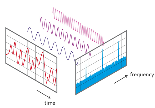\n\n\nAn audio signal is a representation of sound, typically using either a level of electrical voltage for analog signals, or a series of binary numbers for digital signals.\n
\nThey have some important parameters like :\n
\n\n> * Frequency :> Frequency is the number of occurrences of a repeating event per unit of time, measured in hertz (Hz)\n> * Bandwidth :> Bandwidth is the amount of data that can be transferred from one point to another within a network in a specific amount of time,measured in bits per second\n> * The period is the duration of time of one cycle in a repeating event, reciprocal of the frequency\n> * Pitch relates to how high or low the sound is, which in turn depends on the frequency of the vibration\n> * Sampling rate :> Number of samples per second (or per other unit) taken from a continuous signal to make a discrete or digital signal\n> * Bitrate :> refers to the number of bits or the amount of data that are processed over a certain amount of time \n\nand many more...","execution_count":null},{"metadata":{},"cell_type":"markdown","source":"\nLet's try an audio sample now..","execution_count":null},{"metadata":{"trusted":true},"cell_type":"code","source":"path = \"../input/birdsong-recognition/train_audio/cacwre/XC11493.mp3\"\nimport IPython.display as ipd\nipd.Audio(path)","execution_count":null,"outputs":[]},{"metadata":{},"cell_type":"markdown","source":"\nVisializing Waveplot\n
\n\n","execution_count":null},{"metadata":{"trusted":true},"cell_type":"code","source":"def load_wave(files): \n counter=1\n for each_file in files: \n x , sr = librosa.load(each_file)\n plt.figure(figsize=(12, 6))\n plt.subplot(5, 1, counter)\n librosa.display.waveplot(x, sr=sr)\n counter+=1\n plt.title(\"FileName: {}, ebird_code : {}\".format(each_file.split(\"/\")[4],each_file.split(\"/\")[5]))\n plt.plot()\n plt.tight_layout()","execution_count":null,"outputs":[]},{"metadata":{"trusted":true},"cell_type":"code","source":"AUDIO_DIR=\"../input/birdsong-recognition/train_audio\"\nebird_code=\"aldfly\"\n\naudio_files_path=glob.glob(AUDIO_DIR +'/'+ ebird_code + '/*.mp3')[:5]\nload_wave(audio_files_path)","execution_count":null,"outputs":[]},{"metadata":{},"cell_type":"markdown","source":"\nFeel free to change ebird_code as per your requirement\n\n","execution_count":null},{"metadata":{},"cell_type":"markdown","source":"\nVisializing Spectrogram\n
\n\n\n\n\nA spectrogram is a visual representation of the spectrum of frequencies of a signal as it varies with time.\n
\nWhen applied to an audio signal, spectrograms are sometimes called sonographs, voiceprints, or voicegrams. \n
\nWhen the data is represented in a 3D plot they may be called waterfalls.\n\n","execution_count":null},{"metadata":{"trusted":true},"cell_type":"code","source":"def load_spec(files): \n counter=1\n for each_file in files: \n x , sr = librosa.load(each_file)\n plt.figure(figsize=(12, 12))\n plt.subplot(5, 1, counter)\n x = librosa.stft(x)\n x = librosa.amplitude_to_db(abs(x))\n librosa.display.specshow(x, sr=sr, x_axis='time', y_axis='hz')\n counter+=1\n plt.title(\"FileName: {}, ebird_code : {}\".format(each_file.split(\"/\")[4],each_file.split(\"/\")[5]))\n plt.colorbar()\n plt.plot()\n plt.tight_layout()","execution_count":null,"outputs":[]},{"metadata":{"trusted":true},"cell_type":"code","source":"AUDIO_DIR=\"../input/birdsong-recognition/train_audio\"\nebird_code=\"aldfly\"\n\naudio_files_path=glob.glob(AUDIO_DIR +'/'+ ebird_code + '/*.mp3')[:5]\nload_spec(audio_files_path)","execution_count":null,"outputs":[]},{"metadata":{},"cell_type":"markdown","source":"\nFeel free to change ebird_code as per your requirement\n\n","execution_count":null},{"metadata":{},"cell_type":"markdown","source":"\nExploring Testing Meta Data\n
\n
\n\nLet's dive to our CSV...\n\n","execution_count":null},{"metadata":{"trusted":true},"cell_type":"code","source":"test_df=pd.read_csv(\"../input/birdsong-recognition/test.csv\", delimiter=',')","execution_count":null,"outputs":[]},{"metadata":{"trusted":true},"cell_type":"code","source":"test_df = pd.read_csv(\"../input/birdsong-recognition/test.csv\", delimiter = ',')\nprint('There are Total {} datapoints in the dataset with {} Features:'.format(test_df.shape[0], test_df.shape[1]))\ntest_df","execution_count":null,"outputs":[]},{"metadata":{},"cell_type":"markdown","source":"\nWhat? Only 3 Rows?\n\n\n\n \n\nOkay, So That's only what we have right now i.e 27% of data. Rest is hidden
\nHmm.. We also have other CSV too but Let's see where it goes..
\n\nAnyways, According to our Description, Our Hidden Test Data :\n> * Consist of approximately 150 recordings in mp3 format, each roughly 10 minutes long\n> * We have 3 Sites\n> * Sites 1 and 2 were labeled in 5 second increments and need matching predictions\n> * Site 3 files are only labeled at the file level. Also, Site 3 has relatively few rows in the test set and needs lower time resolution predictions\n\nTwo example soundscapes from another data source are also provided to illustrate how the soundscapes are labeled and the hidden dataset folder structure ( Audio Files saved in example_test_audio )
\n\nOur Test.csv has :\n> * site :> Site ID\n> * row_id :> ID code for the row.\n> * seconds :> the second ending the time window, if any. Site 3 time windows cover the entire audio file and have null entries for seconds\n> * audio_id :> ID code for the audio file.\n","execution_count":null},{"metadata":{},"cell_type":"markdown","source":"Time to have a look to the remaining CSV files..","execution_count":null},{"metadata":{"trusted":true},"cell_type":"code","source":"test_df_metadata = pd.read_csv('../input/birdsong-recognition/example_test_audio_metadata.csv')\nprint('There are Total {} datapoints in the dataset with {} Features'.format(test_df_metadata.shape[0], test_df_metadata.shape[1]))\ntest_df_metadata.head(3)","execution_count":null,"outputs":[]},{"metadata":{"trusted":true},"cell_type":"code","source":"test_df_summary = pd.read_csv('../input/birdsong-recognition/example_test_audio_summary.csv')\nprint('There are Total {} datapoints in the dataset with {} Features'.format(test_df_summary.shape[0], test_df_summary.shape[1]))\ntest_df_summary.head(3)","execution_count":null,"outputs":[]},{"metadata":{},"cell_type":"markdown","source":"\nEnd Notes\n
\n
\n\nWith this , We end out initial / just a quick look analysis. Don't worry, this notebook is work in progress :)
\nWe'll meet again with some new insights, findings..
\nThank You to all the recordists (not just the Top-20!) and [Cornell Lab of Ornithology’s Center for Conservation Bioacoustics (CCB)](https://www.birds.cornell.edu/ccb/) for this dataset.
\nBit excited for this competition. It's full of learning experiences. And ik, it'll be fun :D","execution_count":null}],"metadata":{"kernelspec":{"language":"python","display_name":"Python 3","name":"python3"},"language_info":{"pygments_lexer":"ipython3","nbconvert_exporter":"python","version":"3.6.4","file_extension":".py","codemirror_mode":{"name":"ipython","version":3},"name":"python","mimetype":"text/x-python"}},"nbformat":4,"nbformat_minor":4}