{"cells":[{"metadata":{},"cell_type":"markdown","source":"\nTable of Contents \n\n1. [Introduction](#1)\n1. [Pandas Profiling](#2)\n1. [Data Analysis Baseline Library (dabl)](#3)\n 1. [Data Cleaning](#31)\n 1. [EDA](#32)\n 1. [Model Building](#33)\n1. [Pycaret](#4)\n 1. [Load dataset](#41)\n 1. [Comparing all models](#42)\n 1. [Create Model](#43)\n 1. [Tune Model](#44)\n 1. [Plot Model](#45)\n 1. [Predict Model](#46)\n 1. [Finalise Model](#47)\n 1. [Predict on unseen data](#48)\n 1. [Deploy Trained Model on cloud](#49)\n 1. [Save & Load Trained Model from cloud](#410)\n1. [datassist](#5)\n1. [AutoViz](#6) \n1. [missingno](#7) \n1. [Conclusion](#8)\n","execution_count":null},{"metadata":{},"cell_type":"markdown","source":"# 1. Introduction
\nAutomated machine learning (AutoML) represents a fundamental shift in the way organizations of all sizes approach machine learning and data science. Applying traditional machine learning methods to real-world business problems is time-consuming, resource-intensive, and challenging. It requires experts in the several disciplines, including data scientists – some of the most sought-after professionals in the job market right now.\n\nMachine learning technology is no longer just for technology geeks but is now understood and used by business users. However, the future growth of this technology continues to be dependent on the availability of skilled ML workers and data science experts. With the current shortage of skilled ML professionals, most businesses do not have the budget nor the resources to invest in trained team proficient in these technologies.\n\nAutomated machine learning changes that, making it easier to build and use machine learning models in the real world by running systematic processes on raw data and selecting models that pull the most relevant information from the data – what is often referred to as “the signal in the noise.” Automated machine learning incorporates machine learning best practices from top-ranked data scientists to make data science more accessible across the organization.\n\nThe answer lies in the emergence of the automated machine learning pipeline technology also known as the AutoML pipeline as shown below \n\n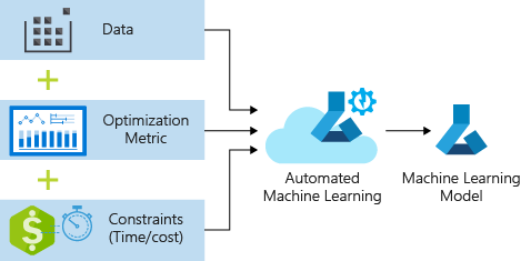\n\nAuto Machine Learning can provide the following benefits:\n\n* Improve productivity of data experts by automating any repetitive ML-related tasks and help them focus on other issues.\n* Reduce human errors in ML models that arise mainly due to manual steps.\n* Make machine learning accessible for all users, thus promoting a decentralized process.","execution_count":null},{"metadata":{},"cell_type":"markdown","source":"# 2. Pandas Profiling
\n\n\nGenerates profile reports from a pandas DataFrame. The pandas df.describe() function is great but a little basic for serious exploratory data analysis. pandas_profiling extends the pandas DataFrame with df.profile_report() for quick data analysis.\n\nFor each column the following statistics - if relevant for the column type - are presented in an interactive HTML report:\n\n* **Type inference**: detect the types of columns in a dataframe.\n* **Essentials**: type, unique values, missing values\n* **Quantile statistics** like minimum value, Q1, median, Q3, maximum, range, interquartile range\n* **Descriptive statistics** like mean, mode, standard deviation, sum, median absolute deviation, coefficient of variation, kurtosis, skewness\n* **Most frequent values**\n* **Histogram**\n* **Correlations** highlighting of highly correlated variables, Spearman, Pearson and Kendall matrices\n* **Missing values** matrix, count, heatmap and dendrogram of missing values\n* **Text analysis** learn about categories (Uppercase, Space), scripts (Latin, Cyrillic) and blocks (ASCII) of text data.\n* **File and Image analysis** extract file sizes, creation dates and dimensions and scan for truncated images or those containing EXIF information.","execution_count":null},{"metadata":{"_kg_hide-output":true,"trusted":true},"cell_type":"code","source":"!pip install pandas-profiling","execution_count":null,"outputs":[]},{"metadata":{"trusted":true},"cell_type":"code","source":"import pandas as pd\nfrom pandas_profiling import ProfileReport\ntrain = pd.read_csv('../input/birdsong-recognition/train.csv')","execution_count":null,"outputs":[]},{"metadata":{"trusted":true},"cell_type":"code","source":"### To Create the Simple report quickly\ntrain.profile_report()","execution_count":null,"outputs":[]},{"metadata":{},"cell_type":"markdown","source":"# 3. Data Analysis Baseline Library (dabl)
\n\nThis project tries to help make supervised machine learning more accessible for beginners, and reduce boiler plate for common tasks.\n\nThis library is in very active development, so it’s not recommended for production use.\nDevelopment at github.com/amueller/dabl.\n\n\nThe idea behind dabl is to jump-start your supervised learning task. dabl has several tools that make it easy to clean and inspect your data, and create strong baseline models.\n\nBuilding machine learning models is an inherently iterative task with a human in the loop. Big jumps in performance are often achieved by better understanding of the data and task, and more appropriate features. dabl tries to provide as much insight into the data as possible, and enable interactive analysis.\n\nMany analyses start with the same rote tasks of cleaning and basic data visualization, and initial modeling. dabl tries to make these steps as easy as possible, so that you can spend your time thinking about the problem and creating more interesting custom analyses.\n\nThere are two main packages that dabl takes inspiration from and that dabl builds upon: scikit-learn and auto-sklearn. The design philosophies and use-cases are quite different, however.\n\nScikit-learn provides many essential building blocks, but is built on the idea to do exactly what the user asks for. That requires specifying every step of the processing in detail. dabl on the other hand has a best-guess philosophy: it tries to do something sensible, and then provides tools for the user to inspect and evaluate the results to judge them.\n\nauto-sklearn is completely automatic and black-box. It searches a vast space of models and constructs complex ensemles of high accuracy, taking a substantial amount of computation and time in the process. The goal of auto-sklearn is to build the best model possible given the data. dabl, conversely, tries to enable the user to quickly iterate and get a grasp on the properties of the data at hand and the fitted models.\n\ndabl is meant to support you in the following tasks, in order:\n## 3.1 Data Cleaning
\n\n**Install dabl**","execution_count":null},{"metadata":{"_kg_hide-output":true,"trusted":true},"cell_type":"code","source":"!pip install dabl","execution_count":null,"outputs":[]},{"metadata":{},"cell_type":"markdown","source":"**Import libraries & Load dataset**","execution_count":null},{"metadata":{"trusted":true},"cell_type":"code","source":"import pandas as pd\nimport dabl\ndf = pd.read_csv(\"../input/house-prices-advanced-regression-techniques/train.csv\")","execution_count":null,"outputs":[]},{"metadata":{},"cell_type":"markdown","source":"Now let’s ask **dabl** what it thinks by cleaning up the data.\n\n**dabl** tries to detect the types of your data and apply appropriate conversions. It also tries to detect potential data quality issues. The field of data cleaning is impossibly broad, and dabl’s approaches are by no means sophisticated. The goal of dabl is to get the data “clean enough” to create useful visualizations and models, and to allow users to perform custom cleaning operations themselves. In particular if the detection of semantic types (continuous, categorical, ordinal, text, etc) fails, the user can provide **type_hints**:","execution_count":null},{"metadata":{"trusted":true},"cell_type":"code","source":"df_clean = dabl.clean(df, verbose=0)","execution_count":null,"outputs":[]},{"metadata":{},"cell_type":"markdown","source":"This provides us with lots of information about what is happening in the different columns. **In this case, we might have been able to figure this out quickly from the call to head, but in larger datasets this might be a bit tricky.** For example we can see that there are several dirty columns with “?” in it. This is probably a marker for a missing value and we could go back and fix our parsing of the CSV, but let’s try and continue with what dabl is doing automatically for now. **In dabl, we can also get a best guess of the column types in a convenient format:**","execution_count":null},{"metadata":{"trusted":true},"cell_type":"code","source":"types = dabl.detect_types(df_clean)\nprint(types) ","execution_count":null,"outputs":[]},{"metadata":{},"cell_type":"markdown","source":"Having a very rough idea of the shape of our data, we can now start looking at the actual content. The easiest way to do that is using visualization of univariate and bivariate patterns. With plot, we can create plot of the features deemed most important for our task.\n\n## 3.2 EDA
\n\n**dabl** provides a high-level interface that summarizes several common high-level plots. For low dimensional datasets, all features are shown; for high dimensional datasets, only the most informative features for the given task are shown. This is clearly not guaranteed to surface all interesting aspects with the data, or to find all data quality issues. However, it will give you a quick insight in to what are the important features, their interactions, and how hard the problem might be. It also allows a good assessment of whether there is any data leakage through spurious representations of the target in the data.","execution_count":null},{"metadata":{"trusted":true},"cell_type":"code","source":"dabl.plot(df, 'SalePrice')","execution_count":null,"outputs":[]},{"metadata":{},"cell_type":"markdown","source":"## 3.3 Model Building
\n\nFinally, we can find an initial model for our data. The SimpleClassifier does all the work for us. It implements the familiar scikit-learn API of fit and predict. Alternatively we could also use the same interface as before and pass the whole data frame and specify the target column.","execution_count":null},{"metadata":{"trusted":true},"cell_type":"code","source":"ec = dabl.SimpleClassifier(random_state=0).fit(df, target_col=\"SalePrice\") ","execution_count":null,"outputs":[]},{"metadata":{},"cell_type":"markdown","source":"The SimpleClassifier first tries several baseline and instantaneous models, potentially on subsampled data, to get an idea of what a low baseline should be. This again is a good place to surface data leakage, as well as find the main discriminative features in the dataset. The SimpleClassifier allows specifying data in the scikit-learn-style fit(X, y) with a 1d y and features X, or with X being a dataframe and specifying the target column inside of X as target_col.\n\nThe SimpleClassifier also performs preprocessing such as missing value imputation and one-hot encoding. ","execution_count":null},{"metadata":{},"cell_type":"markdown","source":"# 4. PyCaret
\n\n\nPyCaret is an open source, low-code machine learning library in Python that allows you to go from preparing your data to deploying your model within seconds in your choice of notebook environment\n\n**Install pycaret**","execution_count":null},{"metadata":{"trusted":true,"_kg_hide-output":true},"cell_type":"code","source":"!pip install pycaret","execution_count":null,"outputs":[]},{"metadata":{},"cell_type":"markdown","source":"## 4.1 Load Dataset
\n\nTo demonstrate the pycaret capability we will use a dataset from UCI called **Default of Credit Card Clients Dataset**. This dataset contains information on default payments, demographic factors, credit data, payment history, and billing statements of credit card clients in Taiwan from April 2005 to September 2005. There are 24,000 samples and 25 features. Short descriptions of each column are as follows:\n\n- **ID:** ID of each client\n- **LIMIT_BAL:** Amount of given credit in NT dollars (includes individual and family/supplementary credit)\n- **SEX:** Gender (1=male, 2=female)\n- **EDUCATION:** (1=graduate school, 2=university, 3=high school, 4=others, 5=unknown, 6=unknown)\n- **MARRIAGE:** Marital status (1=married, 2=single, 3=others)\n- **AGE:** Age in years\n- **PAY_0 to PAY_6:** Repayment status by n months ago (PAY_0 = last month ... PAY_6 = 6 months ago) (Labels: -1=pay duly, 1=payment delay for one month, 2=payment delay for two months, ... 8=payment delay for eight months, 9=payment delay for nine months and above)\n- **BILL_AMT1 to BILL_AMT6:** Amount of bill statement by n months ago ( BILL_AMT1 = last_month .. BILL_AMT6 = 6 months ago)\n- **PAY_AMT1 to PAY_AMT6:** Amount of payment by n months ago ( BILL_AMT1 = last_month .. BILL_AMT6 = 6 months ago)\n- **default.payment.next.month:** Default payment (1=yes, 0=no) `Target Column`","execution_count":null},{"metadata":{"trusted":true},"cell_type":"code","source":"import pandas as pd\ndata=pd.read_csv('../input/default-of-credit-card-clients-dataset/UCI_Credit_Card.csv')\ndata.head()","execution_count":null,"outputs":[]},{"metadata":{},"cell_type":"markdown","source":"In order to demonstrate the predict_model() function on unseen data, a sample of 1500 records has been withheld from the original dataset to be used for predictions. This should not be confused with a train/test split as this particular split is performed to simulate a real life scenario. Another way to think about this is that these 1500 records are not available at the time when the machine learning experiment was performed.","execution_count":null},{"metadata":{"trusted":true},"cell_type":"code","source":"dataset = data.sample(frac=0.95, random_state=786).reset_index(drop=True)\ndata_unseen = data.drop(dataset.index).reset_index(drop=True)\n\nprint('Data for Modeling: ' + str(data.shape))\nprint('Unseen Data For Predictions: ' + str(data_unseen.shape))","execution_count":null,"outputs":[]},{"metadata":{},"cell_type":"markdown","source":"PyCaret's classification module (`pycaret.classification`) is a supervised machine learning module which is used for classifying the elements into a binary group based on various techniques and algorithms. \n\nThe PyCaret classification module can be used for Binary or Multi-class classification problems. It has over 18 algorithms and 14 plots to analyze the performance of models. Be it hyper-parameter tuning, ensembling or advanced techniques like stacking, PyCaret's classification module has it all.","execution_count":null},{"metadata":{"trusted":true},"cell_type":"code","source":"#import classification module from pycaret\nfrom pycaret.classification import *\nexp_clf = setup(data=dataset, target=\"default.payment.next.month\")","execution_count":null,"outputs":[]},{"metadata":{},"cell_type":"markdown","source":"Once the setup has been succesfully executed it prints the information grid which contains several important pieces of information. Most of the information is related to the pre-processing pipeline which is constructed when `setup()` is executed. The majority of these features are out of scope for the purposes of this tutorial however a few important things to note at this stage include:\n\n- **session_id :** A pseduo-random number distributed as a seed in all functions for later reproducibility. If no `session_id` is passed, a random number is automatically generated that is distributed to all functions. \n
\n- **Target Type :** Binary or Multiclass. The Target type is automatically detected and shown. There is no difference in how the experiment is performed for Binary or Multiclass problems. All functionalities are identical.
\n
\n- **Label Encoded :** When the Target variable is of type string (i.e. 'Yes' or 'No') instead of 1 or 0, it automatically encodes the label into 1 and 0 and displays the mapping (0 : No, 1 : Yes) for reference. In this experiment no label encoding is required since the target variable is of type numeric.
\n
\n- **Original Data :** Displays the original shape of the dataset. In this experiment (28500, 25) means 28500 samples and 25 features including the target column.
\n
\n- **Missing Values :** When there are missing values in the original data this will show as True. For this experiment there are no missing values in the dataset. \n
\n
\n- **Numeric Features :** The number of features inferred as numeric. In this dataset, 15 out of 25 features are inferred as numeric.
\n
\n- **Categorical Features :** The number of features inferred as categorical. In this dataset, 9 out of 25 features are inferred as categorical.
\n
\n- **Transformed Train Set :** Displays the shape of the transformed training set. Notice that the original shape of (28500, 25) is transformed into (5984, 90) for the transformed train set and the number of features have increased to 90 from 25 due to categorical encoding
\n
\n- **Transformed Test Set :** Displays the shape of the transformed test/hold-out set. There are 2566 samples in test/hold-out set. This split is based on the default value of 70/30 that can be changed using the `train_size` parameter in setup.
\n\nNotice how a few tasks that are imperative to perform modeling are automatically handled such as missing value imputation (in this case there are no missing values in the training data, but we still need imputers for unseen data), categorical encoding etc. Most of the parameters in `setup()` are optional and used for customizing the pre-processing pipeline. \n\n## 4.2 Comparing all models
\nComparing all models to evaluate performance is the recommended starting point for modeling once the setup is completed (unless you exactly know what kind of model you need, which is often not the case). This function trains all models in the model library and scores them using stratified cross validation for metric evaluation. The output prints a score grid that shows average Accuracy, AUC, Recall, Precision, F1 and Kappa accross the folds (10 by default) of all the available models in the model library.","execution_count":null},{"metadata":{"trusted":true},"cell_type":"code","source":"compare_models()","execution_count":null,"outputs":[]},{"metadata":{},"cell_type":"markdown","source":"There you go created over 15 models using 10 fold stratified cross validation and evaluated the 6 most commonly used classification metrics (Accuracy, AUC, Recall, Precision, F1, Kappa). The score grid printed above highlights the highest performing metric for comparison purposes only. The grid by default is sorted using 'Accuracy' (highest to lowest) which can be changed by passing the sort parameter. For example **compare_models(sort = 'Recall')** will sort the grid by Recall instead of Accuracy. If you want to change the fold parameter from the default value of 10 to a different value then you can use the fold parameter. For example **compare_models(fold = 5)** will compare all models on 5 fold cross validation. Reducing the number of folds will improve the training time.\n## 4.3 Create model
\nWhile compare_models() is a powerful function and often a starting point in any experiment, it does not return any trained models. PyCaret's recommended experiment workflow is to use compare_models() right after setup to evaluate top performing models and finalize a few candidates for continued experimentation. As such, the function that actually allows to you create a model is unimaginatively called **create_model()**.\n\nThere are 18 classifiers available in the model library of PyCaret. \n\nFor illustration purposes only we will be considering the following Classifiers .\n\n* Logistic Regression('lr')\n* Decision Tree Classifier ('dt')\n* K Neighbors Classifier ('knn')\n* Random Forest Classifier ('rf')","execution_count":null},{"metadata":{"trusted":true},"cell_type":"code","source":"lr = create_model('lr')","execution_count":null,"outputs":[]},{"metadata":{"trusted":true},"cell_type":"code","source":"dt = create_model('dt')","execution_count":null,"outputs":[]},{"metadata":{"trusted":true},"cell_type":"code","source":"knn = create_model('knn')","execution_count":null,"outputs":[]},{"metadata":{"trusted":true},"cell_type":"code","source":"rf = create_model('rf')","execution_count":null,"outputs":[]},{"metadata":{},"cell_type":"markdown","source":"Notice that the mean score of all models matches with the score printed in compare_models(). This is because the metrics printed in the compare_models() score grid are the average scores across all CV folds. Similar to compare_models(), if you want to change the fold parameter from the default value of 10 to a different value then you can use the fold parameter. For Example: create_model('dt', fold = 5) will create a Decision Tree Classifier using 5 fold stratified CV.\n## 4.4 Tune model
\nWhen a model is created using the create_model() function it uses the default hyperparameters. In order to tune hyperparameters, the tune_model() function is used. This function automatically tunes the hyperparameters of a model on a pre-defined search space and scores it using stratified cross validation. The output prints a score grid that shows Accuracy, AUC, Recall, Precision, F1 and Kappa by fold.\n\nNow let us tune the below models \n* Logistic Regression('lr')\n* Decision Tree Classifier ('dt')\n* K Neighbors Classifier ('knn')\n* Random Forest Classifier ('rf')","execution_count":null},{"metadata":{"trusted":true},"cell_type":"code","source":"# Tune the Logistic regression model\ntuned_lr = tune_model('lr')","execution_count":null,"outputs":[]},{"metadata":{"trusted":true},"cell_type":"code","source":"# Tune the Decision Tree Classifier model\ntuned_dt = tune_model('dt')","execution_count":null,"outputs":[]},{"metadata":{"trusted":true},"cell_type":"code","source":"# Tune the K Neighbors Classifier model\ntuned_knn = tune_model('knn')","execution_count":null,"outputs":[]},{"metadata":{"trusted":true},"cell_type":"code","source":"# Tune the Random Forest Classifier model\ntuned_rf = tune_model('rf')","execution_count":null,"outputs":[]},{"metadata":{},"cell_type":"markdown","source":"**Note:**\n\nNotice how the results after tuning have been improved:\n\n* Logistic Regression(Before: 0.7786 , After: 0.7786)\n* Decision Tree Classifier (Before: 0.7216 , After: 0.7413)\n* K Neighbors Classifier (Before: 0.7355 , After: 0.7772)\n* Random Forest Classifier (Before: 0.8015 , After: 0.8103)\n\n## 4.5 Plot Model
\n\nBefore model finalization, the `plot_model()` function can be used to analyze the performance across different aspects such as AUC, confusion_matrix, decision boundary etc. This function takes a trained model object and returns a plot based on the test / hold-out set. \n\nThere are 15 different plots available.","execution_count":null},{"metadata":{"trusted":true},"cell_type":"code","source":"#Plot LR model: ROC-AUC curve\nplot_model(lr)","execution_count":null,"outputs":[]},{"metadata":{"trusted":true},"cell_type":"code","source":"#Plot LR model: ROC-AUC curve\nplot_model(tuned_lr)","execution_count":null,"outputs":[]},{"metadata":{"trusted":true},"cell_type":"code","source":"#Plot Decision Tree model: ROC-AUC curve\nplot_model(dt)","execution_count":null,"outputs":[]},{"metadata":{"trusted":true},"cell_type":"code","source":"#Plot KNN model: ROC-AUC curve\nplot_model(knn)","execution_count":null,"outputs":[]},{"metadata":{},"cell_type":"markdown","source":"To analyze the performance of models is to use the **evaluate_model()** function which displays a user interface for all of the available plots for a given model. It internally uses the plot_model() function.","execution_count":null},{"metadata":{"trusted":true},"cell_type":"code","source":"evaluate_model(lr)","execution_count":null,"outputs":[]},{"metadata":{"trusted":true},"cell_type":"code","source":"#create a tree base model to interpret model and check feature importance\ndt = create_model('dt')\n#interpret a model\ninterpret_model(dt)","execution_count":null,"outputs":[]},{"metadata":{"trusted":true},"cell_type":"code","source":"#optimize threshold for trained LR model\noptimize_threshold(lr)","execution_count":null,"outputs":[]},{"metadata":{},"cell_type":"markdown","source":"## 4.6 Predict
\nNow, using our final trained model stored in the tuned_rf variable we will predict against the hold-out sample and evaluate the metrics to see if they are materially different than the CV results.","execution_count":null},{"metadata":{"trusted":true},"cell_type":"code","source":"predict_model(tuned_rf);","execution_count":null,"outputs":[]},{"metadata":{},"cell_type":"markdown","source":"## 4.7 Finalise Trained Model
\nModel finalization is the last step in the experiment. A normal machine learning workflow in PyCaret starts with setup(), followed by comparing all models using compare_models() and shortlisting a few candidate models (based on the metric of interest) to perform several modeling techniques such as hyperparameter tuning, ensembling, stacking etc. This workflow will eventually lead you to the best model for use in making predictions on new and unseen data. The finalize_model() function fits the model onto the complete dataset including the test/hold-out sample (30% in this case). The purpose of this function is to train the model on the complete dataset before it is deployed in production.\n\nOnce the model is finalized using finalize_model(), the entire dataset including the test/hold-out set is used for training. ","execution_count":null},{"metadata":{"trusted":true},"cell_type":"code","source":"final_rf = finalize_model(tuned_rf)","execution_count":null,"outputs":[]},{"metadata":{},"cell_type":"markdown","source":"## 4.8 Predict on unseen data
\nThe predict_model() function is also used to predict on the unseen dataset. The only difference from section 11 above is that this time we will pass the data_unseen parameter. data_unseen is the variable created at the beginning of the tutorial and contains 5% (1500 samples) of the original dataset which was never exposed to PyCaret.","execution_count":null},{"metadata":{"trusted":true},"cell_type":"code","source":"unseen_predictions = predict_model(final_rf, data=data_unseen)\nunseen_predictions.head()","execution_count":null,"outputs":[]},{"metadata":{},"cell_type":"markdown","source":"The Label and Score columns are added onto the data_unseen set. Label is the prediction and score is the probability of the prediction.We have now finished the experiment by finalizing the tuned_rf model which is now stored in final_rf variable. We have also used the model stored in final_rf to predict data_unseen. \n\n## 4.9 Deploy Trained Model on cloud
","execution_count":null},{"metadata":{"trusted":true},"cell_type":"code","source":"deploy_model(model = tuned_rf, model_name = 'deploy_lr', platform = 'flask', authentication = {'bucket' : 'pycaret-test'})","execution_count":null,"outputs":[]},{"metadata":{},"cell_type":"markdown","source":"## 4.10 Save & Load Trained Model from cloud
\n\nTo load a saved model at a future date in the same or an alternative environment, we would use PyCaret's load_model() function and then easily apply the saved model on new unseen data for prediction.","execution_count":null},{"metadata":{"trusted":true},"cell_type":"code","source":"save_model(tuned_rf, 'tuned_rf_16072020')","execution_count":null,"outputs":[]},{"metadata":{"trusted":true},"cell_type":"code","source":"# Load the saved model\nsaved_rf = load_model('tuned_rf_16072020')","execution_count":null,"outputs":[]},{"metadata":{"trusted":true},"cell_type":"code","source":"# Save the experiment\nsave_experiment('experiment_16072020')","execution_count":null,"outputs":[]},{"metadata":{"trusted":true},"cell_type":"code","source":"# Load experiment\nsaved_experiment = load_experiment('experiment_16072020')","execution_count":null,"outputs":[]},{"metadata":{},"cell_type":"markdown","source":"# 5.datasist
\n\n**datasist** is a python package providing fast, quick, and an abstracted interface to popular and frequently used functions or techniques relating to data analysis, visualization, data exploration, feature engineering, Computer, NLP, Deep Learning, modeling, model deployment etc.","execution_count":null},{"metadata":{"trusted":true,"_kg_hide-output":true},"cell_type":"code","source":"!pip install datasist","execution_count":null,"outputs":[]},{"metadata":{"trusted":true},"cell_type":"code","source":"import pandas as pd\nimport datasist as ds #import datasist library\nimport numpy as np\n\ntrain_df = pd.read_csv('../input/house-prices-advanced-regression-techniques/train.csv')\ntest_df = pd.read_csv('../input/house-prices-advanced-regression-techniques/test.csv')","execution_count":null,"outputs":[]},{"metadata":{},"cell_type":"markdown","source":"**check_train_test_set**: Checks the distribution of train and test for uniqueness in order to determine the best feature engineering strategy.","execution_count":null},{"metadata":{"trusted":true},"cell_type":"code","source":"ds.structdata.check_train_test_set(train_df, test_df, index=None, col=None)","execution_count":null,"outputs":[]},{"metadata":{},"cell_type":"markdown","source":"**describe:** Calculates statistics and information about a data set. Information displayed are shapes, size, number of categorical/numeric/date features, missing values, dtypes of objects etc.","execution_count":null},{"metadata":{"trusted":true},"cell_type":"code","source":"ds.structdata.describe(train_df)","execution_count":null,"outputs":[]},{"metadata":{"trusted":true},"cell_type":"code","source":"ds.structdata.describe(test_df)","execution_count":null,"outputs":[]},{"metadata":{},"cell_type":"markdown","source":"**detect_outliers**: Detect Rows with outliers.","execution_count":null},{"metadata":{"trusted":true},"cell_type":"code","source":"numerical_feats = ds.structdata.get_num_feats(train_df)\nds.structdata.detect_outliers(train_df,80,numerical_feats)","execution_count":null,"outputs":[]},{"metadata":{},"cell_type":"markdown","source":"**display_missing**: Display missing values as a pandas dataframe.","execution_count":null},{"metadata":{"trusted":true},"cell_type":"code","source":"ds.structdata.display_missing(train_df)","execution_count":null,"outputs":[]},{"metadata":{"trusted":true},"cell_type":"code","source":"ds.structdata.display_missing(test_df)","execution_count":null,"outputs":[]},{"metadata":{},"cell_type":"markdown","source":"**get_cat_feats** : Returns the categorical features in a data set","execution_count":null},{"metadata":{"trusted":true},"cell_type":"code","source":"cat_feats = ds.structdata.get_cat_feats(train_df)\ncat_feats","execution_count":null,"outputs":[]},{"metadata":{},"cell_type":"markdown","source":"**get_num_feats** : Returns the numerical features in a data set","execution_count":null},{"metadata":{"trusted":true},"cell_type":"code","source":"num_feats = ds.structdata.get_num_feats(train_df)\nnum_feats","execution_count":null,"outputs":[]},{"metadata":{"trusted":true},"cell_type":"code","source":"get_unique_counts = ds.structdata.get_unique_counts(train_df)\nget_unique_counts","execution_count":null,"outputs":[]},{"metadata":{},"cell_type":"markdown","source":"","execution_count":null},{"metadata":{"trusted":true},"cell_type":"code","source":"ds.visualizations.autoviz(train_df)","execution_count":null,"outputs":[]},{"metadata":{"trusted":true},"cell_type":"code","source":"all_data, ntrain, ntest = ds.structdata.join_train_and_test(train_df, test_df)\nprint(\"New size of combined data {}\".format(all_data.shape))\nprint(\"Old size of train data: {}\".format(ntrain))\nprint(\"Old size of test data: {}\".format(ntest))\n\n#later splitting after transformations\ntrain = all_data[:ntrain]\ntest = all_data[ntrain:]","execution_count":null,"outputs":[]},{"metadata":{"trusted":true},"cell_type":"code","source":"new_train_df = ds.feature_engineering.drop_missing(train_df, \n percent=7.0)\nds.structdata.display_missing(new_train_df)","execution_count":null,"outputs":[]},{"metadata":{"trusted":true},"cell_type":"code","source":"ds.feature_engineering.drop_redundant(new_train_df)","execution_count":null,"outputs":[]},{"metadata":{"trusted":true},"cell_type":"code","source":"df = ds.feature_engineering.fill_missing_cats(train_df)\nds.structdata.display_missing(df)","execution_count":null,"outputs":[]},{"metadata":{"trusted":true},"cell_type":"code","source":"df = ds.feature_engineering.fill_missing_num(train_df)\nds.structdata.display_missing(df)","execution_count":null,"outputs":[]},{"metadata":{"trusted":true},"cell_type":"code","source":"df = ds.feature_engineering.fill_missing_num(df)\ndf = ds.feature_engineering.log_transform(df,columns=['Id'])","execution_count":null,"outputs":[]},{"metadata":{},"cell_type":"markdown","source":"# 6.AutoViz
\n\nAutomatically Visualize any dataset, any size with a single line of code.\n\nAutoViz performs automatic visualization of any dataset with one line. Give any input file (CSV, txt or json) and AutoViz will visualize it.","execution_count":null},{"metadata":{"_kg_hide-output":true,"trusted":true},"cell_type":"code","source":"!pip install autoviz","execution_count":null,"outputs":[]},{"metadata":{"trusted":true},"cell_type":"code","source":"import pandas as pd\nfrom autoviz.AutoViz_Class import AutoViz_Class\nAV = AutoViz_Class()","execution_count":null,"outputs":[]},{"metadata":{"trusted":true},"cell_type":"code","source":"sep = ','\ntarget = 'medv'\ndatapath = ''\nfilename = 'https://raw.githubusercontent.com/vincentarelbundock/Rdatasets/master/csv/MASS/Boston.csv'\ndft = AV.AutoViz(datapath+filename, sep=sep, depVar=target, dfte=df, header=0, verbose=2,\n lowess=False,chart_format='svg',max_rows_analyzed=1500,max_cols_analyzed=30)","execution_count":null,"outputs":[]},{"metadata":{},"cell_type":"markdown","source":"# 7. missingno
\n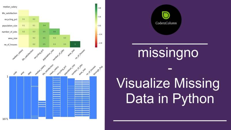\nMessy datasets? Missing values? missingno provides a small toolset of flexible and easy-to-use missing data visualizations and utilities that allows you to get a quick visual summary of the completeness (or lack thereof) of your dataset. Just pip install missingno to get started.\n\nIn the case of a real-world dataset, it is very common that some values in the dataset are missing. We represent these missing values as NaN (Not a Number) values. But to build a good machine learning model our dataset should be complete. That’s why we use some imputation techniques to replace the NaN values with some probable values. But before doing that we need to have a good understanding of how the NaN values are distributed in our dataset.\n\nMissingno library offers a very nice way to visualize the distribution of NaN values. Missingno is a Python library and compatible with Pandas.","execution_count":null},{"metadata":{"_kg_hide-output":true,"trusted":true},"cell_type":"code","source":"!pip install missingno","execution_count":null,"outputs":[]},{"metadata":{"trusted":true},"cell_type":"code","source":"import missingno as msno\nimport pandas as pd\nimport numpy as np\n\ntrain_df = pd.read_csv('../input/titanic/train.csv')","execution_count":null,"outputs":[]},{"metadata":{},"cell_type":"markdown","source":"**Matrix:**\n\nVisualising missing values for a sample of 150 Using this matrix you can very quickly find the pattern of missingness in the dataset.","execution_count":null},{"metadata":{"trusted":true},"cell_type":"code","source":"msno.matrix(train_df.sample(100))","execution_count":null,"outputs":[]},{"metadata":{},"cell_type":"markdown","source":"**Heatmap**\n\nThe missingno correlation heatmap measures nullity correlation: how strongly the presence or absence of one variable affects the presence of another:","execution_count":null},{"metadata":{"trusted":true},"cell_type":"code","source":"msno.heatmap(train_df)","execution_count":null,"outputs":[]},{"metadata":{},"cell_type":"markdown","source":"**Bar Chart :**\n\nThis bar chart gives you an idea about how many missing values are there in each column.","execution_count":null},{"metadata":{"trusted":true},"cell_type":"code","source":"msno.bar(train_df.sample(880))","execution_count":null,"outputs":[]},{"metadata":{},"cell_type":"markdown","source":"**Dendogram:**\n\nThe dendrogram uses a hierarchical clustering algorithm (courtesy of scipy) to bin variables against one another by their nullity correlation (measured in terms of binary distance). At each step of the tree the variables are split up based on which combination minimizes the distance of the remaining clusters. The more monotone the set of variables, the closer their total distance is to zero, and the closer their average distance (the y-axis) is to zero.\n\nTo interpret this graph, read it from a top-down perspective. Cluster leaves which linked together at a distance of zero fully predict one another's presence—one variable might always be empty when another is filled, or they might always both be filled or both empty, and so on. In this specific example the dendrogram glues together the variables which are required and therefore present in every record.\n\nCluster leaves which split close to zero, but not at it, predict one another very well, but still imperfectly. If your own interpretation of the dataset is that these columns actually are or ought to be match each other in nullity , then the height of the cluster leaf tells you, in absolute terms, how often the records are \"mismatched\" or incorrectly filed—that is, how many values you would have to fill in or drop, if you are so inclined.\n\nAs with matrix, only up to 50 labeled columns will comfortably display in this configuration. However the dendrogram more elegantly handles extremely large datasets by simply flipping to a horizontal configuration.","execution_count":null},{"metadata":{"trusted":true},"cell_type":"code","source":"msno.dendrogram(train_df)","execution_count":null,"outputs":[]},{"metadata":{"_uuid":"2ee8624d8356a00b939c3eb92e2ecd399d9f0db5"},"cell_type":"markdown","source":"# Conclusion
\n\nHence Automated ML tools is enabling data scientists to improve their productivity and realize their true potential quickly and time to market with quicker insights. I hope you find this kernel useful and will use the above tools to good effect in your day to day data science career path.\n\n# If you like this kernel greatly appreciate to UPVOTE ","execution_count":null}],"metadata":{"kernelspec":{"language":"python","display_name":"Python 3","name":"python3"},"language_info":{"pygments_lexer":"ipython3","nbconvert_exporter":"python","version":"3.6.4","file_extension":".py","codemirror_mode":{"name":"ipython","version":3},"name":"python","mimetype":"text/x-python"}},"nbformat":4,"nbformat_minor":4}