{"metadata":{"kernelspec":{"language":"python","display_name":"Python 3","name":"python3"},"language_info":{"pygments_lexer":"ipython3","nbconvert_exporter":"python","version":"3.6.4","file_extension":".py","codemirror_mode":{"name":"ipython","version":3},"name":"python","mimetype":"text/x-python"}},"nbformat_minor":4,"nbformat":4,"cells":[{"cell_type":"markdown","source":"\n# **🐤🐦Introduction - Bird song/Birdcall recognition🔉🔉** ","metadata":{}},{"cell_type":"markdown","source":"### Bioacoutics era why and how birds are useful for our environment !\nEcosystem services are natural processes that improves the quality of humans life. Birds contribute to many positive benefits as recognized by Cornell lab of Ornitology - the goal is to advance the understanding and protection of the natural world by provisioning, regulating, cultural, and supporting. They focus primarily on supporting services and to a lesser extent on provisioning and regulating services. As members of ecosystems, birds play many roles, including predator, pollinator, scavenger, seed disperser, seed predator, and ecosystem engineer. \n\nThese ecosystem services fall into two subcategories: \n 1. Those that result from bird behavior (such as consuming agricultural pests) and those that result from bird products (such as nests and guano).\n 2. Most birds have characteristics that make them special from an ecosystem services perspective. Because most birds fly, they can respond to irregular or pulsatile resources in ways that other vertebrates generally cannot. Migratory bird species connect ecosystem processes and flows that are separated by great distances and times. \n\nThe Cornell Lab of Ornithology combines the agility and impact of a local nonprofit organization with world-class science and teaching as part of Cornell College’s College of Agriculture and Life Sciences. Our work spans disciplines from science to art, engineering to education. Our global community includes supporters, participants, and partners from all walks of life, united by a love of birds and nature and a commitment to protecting the planet.\n\nThere are already numerous projects to comprehensively monitor birds by continuously recording natural soundscapes over long periods of time. However, because many living and non-living things produce sounds, analysis of these data sets is often done manually by professionals. These analyses are tedious and slow, and the results are often incomplete. Data science can remedy this, and so researchers have turned to large crowdsourced databases of focal recordings of birds to train AI models.","metadata":{}},{"cell_type":"markdown","source":"* [Introduction - Introduction - Bird song/Birdcall recognition](#section-one)\n* [Challenges in Birdclef competiton](#section-two)\n* [Data Preprocessing from writups](#section-three)\n* [Simple EDA and Data visualiation](#section-four)\n* [Data Augmentations](#section-five)\n* [Model Architectures In BirdCLEF series](#section-six)\n* [loss functions](#section-seven)\n* [Solution Writeups](#section-eight)\n* [Conclusion](#section-nine)\n* [References](#section-ten)\n* [Submission Process](#section-eleven)","metadata":{}},{"cell_type":"markdown","source":"\n# **Challenges in Birdclef competition** ","metadata":{}},{"cell_type":"markdown","source":"The Main challenge is there are disconnect between the training (Short Audios from Xenocanto) datas and test data (soundscape recordings - long recordings with multiple species and other sounds used in monitoring applications).\n\n - **Birdclef 2020** : Key focuses on the identification of 264 bird species using training data from Xenocanto recordings and test data was populated with approximately 150 mp3 recordings roughly 10 minutes long. The test data was recorded in 3 different site locations from north america\n - **Birdclef 2021** : Key focuses on the identification of 397 bird species using training data from Xenocanto recordings and test data was populated with approximately 80 ogg recordings roughly 10 minutes long. The test data was recorded from 4 different locations namely COL (Jardín,Departamento de Antioquia, Colombia), COR (Alajuela, SanRamón, Costa Rica), SNE (Sierra Nevada, California, USA),and SSW (Ithaca, New York, USA)\n - **Birdclef 2022** : Key focus was to monitor rare birds in Hawaii. The training data comprises of 152 bird species from Xenocanto recordings and test data conatins primary focus on 21 species namely \"akiapo\", \"aniani\", \"apapan\", \"barpet\", \"crehon\", \"elepai\", \"ercfra\", \"hawama\", \"hawcre\", \"hawgoo\", \"hawhaw\", \"hawpet1\", \"houfin\", \"iiwi\", \"jabwar\", \"maupar\", \"omao\", \"puaioh\", \"skylar\", \"warwhe1\", \"yefcan\" recorded in Hawaii.\n - **Birdclef 2023** : Key focus was to monitor birds in Kenya. The training data comprises of 264 imbalance bird species from Xenocanto recordings and test data was populated with approximately 200 ogg recordings roughly 10 minutes long.","metadata":{}},{"cell_type":"code","source":"import numpy as np # linear algebra\nimport pandas as pd # data processing, CSV file I/O (e.g. pd.read_csv)\nimport os\n#import audiomentations\nfrom glob import glob\nfrom tqdm import tqdm\ntqdm.pandas() # enable progress bars in pandas operations\nimport gc\nimport librosa\nimport sklearn\nimport json\n# Import for visualization\nimport matplotlib as mpl\ncmap = mpl.cm.get_cmap('coolwarm')\nimport matplotlib.pyplot as plt\nimport librosa.display as lid\nimport IPython.display as ipd\nimport cv2\nimport tensorflow as tf\nimport librosa\nimport librosa.display as lid\n","metadata":{"_kg_hide-input":true,"execution":{"iopub.status.busy":"2023-06-18T10:37:51.357821Z","iopub.execute_input":"2023-06-18T10:37:51.358444Z","iopub.status.idle":"2023-06-18T10:38:02.337758Z","shell.execute_reply.started":"2023-06-18T10:37:51.358408Z","shell.execute_reply":"2023-06-18T10:38:02.336503Z"},"trusted":true},"execution_count":null,"outputs":[]},{"cell_type":"markdown","source":"\n# **Data Preprocessing from top score writups** \n- **PSI** : Mel spectrogram representation of a 30 sec wav-crop as input for training. Inference used 5 second clip \n- **SHIRO** : Mel spectrogram representation of a 20 sec wav-crop as input. Inference used 5 second clip\n- **TATTAKA** : Mel spectrogram representation of a minimum 30/20 sec wav-crop as input. Inference used 5 second clip.\n- **VOLODYMYR** : Mel spectrogram representation of a minimum 15 sec wav-crop as input. Inference used 5 second clip.\n- **SLIME** : Mel spectrogram representation of a minimum 20/30 sec wav-crop as input. Inference used 5 second clip.\n- **KRAMARENKO VLADISLAV** : Mel spectrogram representation of a minimum 2.5 sec wav-crop as input. Inference used 5 second clip.\n- **2023Clef** : Average Input audio file used was minimum of 10 to 30 secs\n\n\n **MelSpectrograms Features overall**\n- **Sampling Rate** = 32000/21000\n- **n_mels** =128\n- **f_min**=50\n- **f_max**=15000\n- **n_fft**=2048\n- **hop_length**=512\n\n","metadata":{}},{"cell_type":"markdown","source":" \n
\n ","metadata":{}},{"cell_type":"markdown","source":"Data Augmenrtations plays a major role in BirdCLEF competitions. Here are the list of augmentations its explanation and visualization\n\n1. **Gaussian noise**: Gaussian noise is added with randomly chosen weights to the audio signal while renormalizing the results \n2. **Background**: pink noise. Background noise in the form of pink noise is added. The pink noise is generated using the python library colorednoise4. Adding background noise is a so-called mix up augmentation method where the labels of the background noise are neglected (Fig. 3c) (Audiomentations: function\n3. **Background**: noise soundscapes. The background\n noise is noise data extracted from soundscapes.\n Adding background noise is a mix up augmentations\n method where the labels of the background noise\n are neglected \n \n4. **General mix up**: Training examples are constructed\n using the following equation:\n x = xi + (1−τ )·xj (1)\n where xi and xj are the two randomly selected samples\n from the training data, for which τ is the mix up’s\n ratio (Fig. 3e). The Pytorch Image Models (timm)’s\n mixup() function is utilized5.\n \n5. **Horizontal roll**: This method is applied to the spectrograms. It rolls the spectrogram with respect to\n width × α, whereas α is the roll factor (e.g., 0.5)\n\n6. **Vertical roll**: This method is applied to the spectrograms. It rolls the spectrogram with respect to\n height × α, whereas α is the roll factor (e.g., 0.05)\n\n7. **Pitch shift**: Shifts the pitch of the sound up or down\n without changing the audio’s pace. For a random\n pitch shift, the shift is realized based on a pitch factor.\n 5Pytorch Image Models (timm): Mixup & CutMix Augmentations, https://timm.fast.ai/mixup_cutmix\n When the pitch factor is less than zero, a downwards\n shift is realized, whereby a factor greater than zero\n shifts upwards.\n8. **Time mask**: t consecutive time steps are masked,\n whereas t is chosen from a uniform normal distribution ∈ {t0,··· ,T} with the time mask parameter T,\n for which t0 ∈ {0, τ − t}.\n \n9. **Frequency mask**: f consecutive mel frequency channels from {f0,··· ,f0 + f} are masked, whereas f\n is chosen from an uniform normal distribution ∈\n {0,··· ,F} with the frequency masking parameter F,\n for which f0 ∈ {0,v −f} with v being the number of\n mel frequency bands .\n10. **Gain**: Multiplies the audio signal by a random amplitude factor in order to reduce or increase the present\n volume. This technique can help a model to approach invariance to the overall gain of the input audio.\n \n11. **Loudness normalization**: Applies a constant amount of gain to match a specific loudness. \n\n12. **Horizontal flip**: The spectrogram is horizontally\n flipped along the y-axis.\n \n13. **Vertical flip**: The spectrogram is vertically flipped\n along the x-axis.\n \n14. **Time stretch**: Stretches the signal in time without\n changing the signal’s pitch. For time stretch factors greater than 1, the signal sped up, whereby factors less than 0 result in a slowing down of the pace. For application, the rate factor is randomly sampled\n from [0.9,1.5]. \n15. **Blurring**: An average blur filter is used with a kernel size of 3 × 3 by utilizing the Open Source Computer Vision Library OpenCV6\n\n16. **Cropping**: Randomly selects values for the top, bottom, left, and right parts of the spectrogram. Finally, a\n cropping and a resizing of the spectrogram with respect\n to its original aspect ratio is realized (Fig. 3s) (baseline\n system.\n17. **tanh-based distortion**: This technique adds tanh-based\n distortion to the audio recording. The hyperbolic tangent functionality can provide a soft clipping, whereas\n the distortion’s magnitude is proportional to the loudness of the input and the pre-gain. As the hyperbolic\n tangent is symmetric, the positive and the negative parts\n of the signal are equally squashed.","metadata":{}},{"cell_type":"markdown","source":"
 \n
\nAudiomentations image visualization
","metadata":{}},{"cell_type":"markdown","source":"\n## Model Architectures In BirdCLEF series\nSED the task differs from the tasks in past audio contests in kaggle. The task in Freesound Audio Tagging 2019, Freesound General-Purpose Audio Tagging Challenge is audio tagging, for which we need to provide a clip-level prediction, and the task in TensorFlow Speech Recognition Challenge is speech recognition, so we need to predict what speech command is in this audio clip (which is similar to the audio tagging task in a sense, as we only need to provide a clip-level prediction. SED tasks mostly used in [DCASE 2018-2023 ](https://dcase.community/challenge2021/task-sound-event-detection-and-separation-in-domestic-environments) competitions which acted as a base in BirdCLEF competitions, The Famous repository name [PANNs models](https://github.com/qiuqiangkong/audioset_tagging_cnn/blob/master/pytorch/models.py) \n\n \n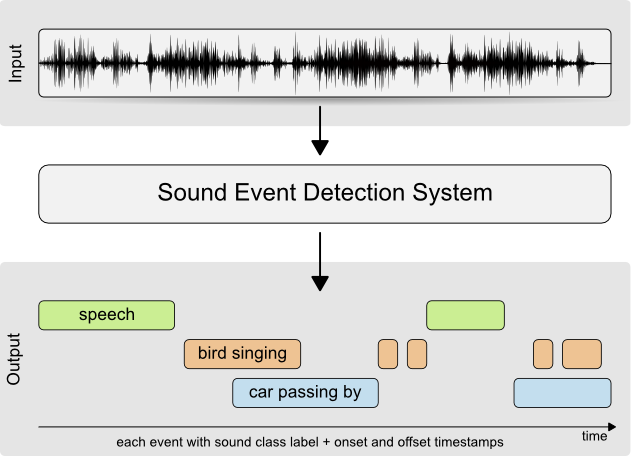\n\n**Most of the top performers in BirdCLEF competitions below is baseline architecture used thanks to HIDEHISA ARAI for providing such a baseline model**\n\n\n def init_layer(layer):\n nn.init.xavier_uniform_(layer.weight)\n\n if hasattr(layer, \"bias\"):\n if layer.bias is not None:\n layer.bias.data.fill_(0.)\n\n\n def init_bn(bn):\n bn.bias.data.fill_(0.)\n bn.weight.data.fill_(1.0)\n\n\n def interpolate(x: torch.Tensor, ratio: int):\n\n (batch_size, time_steps, classes_num) = x.shape\n upsampled = x[:, :, None, :].repeat(1, 1, ratio, 1)\n upsampled = upsampled.reshape(batch_size, time_steps * ratio, classes_num)\n return upsampled\n\n\n def pad_framewise_output(framewise_output: torch.Tensor, frames_num: int):\n \n output = torch.cat((framewise_output, pad), dim=1)\n return output\n\n\n class ConvBlock(nn.Module):\n def __init__(self, in_channels: int, out_channels: int):\n super().__init__()\n\n self.conv1 = nn.Conv2d(\n in_channels=in_channels,\n out_channels=out_channels,\n kernel_size=(3, 3),\n stride=(1, 1),\n padding=(1, 1),\n bias=False)\n\n self.conv2 = nn.Conv2d(\n in_channels=out_channels,\n out_channels=out_channels,\n kernel_size=(3, 3),\n stride=(1, 1),\n padding=(1, 1),\n bias=False)\n\n self.bn1 = nn.BatchNorm2d(out_channels)\n self.bn2 = nn.BatchNorm2d(out_channels)\n\n self.init_weight()\n\n def init_weight(self):\n init_layer(self.conv1)\n init_layer(self.conv2)\n init_bn(self.bn1)\n init_bn(self.bn2)\n\n def forward(self, input, pool_size=(2, 2), pool_type='avg'):\n\n x = input\n x = F.relu_(self.bn1(self.conv1(x)))\n x = F.relu_(self.bn2(self.conv2(x)))\n if pool_type == 'max':\n x = F.max_pool2d(x, kernel_size=pool_size)\n elif pool_type == 'avg':\n x = F.avg_pool2d(x, kernel_size=pool_size)\n elif pool_type == 'avg+max':\n x1 = F.avg_pool2d(x, kernel_size=pool_size)\n x2 = F.max_pool2d(x, kernel_size=pool_size)\n x = x1 + x2\n else:\n raise Exception('Incorrect argument!')\n\n return x\n\n\n class AttBlock(nn.Module):\n def __init__(self,\n in_features: int,\n out_features: int,\n activation=\"linear\",\n temperature=1.0):\n super().__init__()\n\n self.activation = activation\n self.temperature = temperature\n self.att = nn.Conv1d(\n in_channels=in_features,\n out_channels=out_features,\n kernel_size=1,\n stride=1,\n padding=0,\n bias=True)\n self.cla = nn.Conv1d(\n in_channels=in_features,\n out_channels=out_features,\n kernel_size=1,\n stride=1,\n padding=0,\n bias=True)\n\n self.bn_att = nn.BatchNorm1d(out_features)\n self.init_weights()\n\n def init_weights(self):\n init_layer(self.att)\n init_layer(self.cla)\n init_bn(self.bn_att)\n\n def forward(self, x):\n # x: (n_samples, n_in, n_time)\n norm_att = torch.softmax(torch.clamp(self.att(x), -10, 10), dim=-1)\n cla = self.nonlinear_transform(self.cla(x))\n x = torch.sum(norm_att * cla, dim=2)\n return x, norm_att, cla\n\n def nonlinear_transform(self, x):\n if self.activation == 'linear':\n return x\n elif self.activation == 'sigmoid':\n return torch.sigmoid(x)\n \n class PANNsCNN14Att(nn.Module):\n def __init__(self, sample_rate: int, window_size: int, hop_size: int,\n mel_bins: int, fmin: int, fmax: int, classes_num: int):\n super().__init__()\n\n window = 'hann'\n center = True\n pad_mode = 'reflect'\n ref = 1.0\n amin = 1e-10\n top_db = None\n self.interpolate_ratio = 32 # Downsampled ratio\n\n # Spectrogram extractor\n self.spectrogram_extractor = Spectrogram(\n n_fft=window_size,\n hop_length=hop_size,\n win_length=window_size,\n window=window,\n center=center,\n pad_mode=pad_mode,\n freeze_parameters=True)\n\n # Logmel feature extractor\n self.logmel_extractor = LogmelFilterBank(\n sr=sample_rate,\n n_fft=window_size,\n n_mels=mel_bins,\n fmin=fmin,\n fmax=fmax,\n ref=ref,\n amin=amin,\n top_db=top_db,\n freeze_parameters=True)\n\n # Spec augmenter\n self.spec_augmenter = SpecAugmentation(\n time_drop_width=64,\n time_stripes_num=2,\n freq_drop_width=8,\n freq_stripes_num=2)\n\n self.bn0 = nn.BatchNorm2d(mel_bins)\n\n self.conv_block1 = ConvBlock(in_channels=1, out_channels=64)\n self.conv_block2 = ConvBlock(in_channels=64, out_channels=128)\n self.conv_block3 = ConvBlock(in_channels=128, out_channels=256)\n self.conv_block4 = ConvBlock(in_channels=256, out_channels=512)\n self.conv_block5 = ConvBlock(in_channels=512, out_channels=1024)\n self.conv_block6 = ConvBlock(in_channels=1024, out_channels=2048)\n\n self.fc1 = nn.Linear(2048, 2048, bias=True)\n self.att_block = AttBlock(2048, classes_num, activation='sigmoid')\n\n self.init_weight()\n\n def init_weight(self):\n init_bn(self.bn0)\n init_layer(self.fc1)\n \n def cnn_feature_extractor(self, x):\n x = self.conv_block1(x, pool_size=(2, 2), pool_type='avg')\n x = F.dropout(x, p=0.2, training=self.training)\n x = self.conv_block2(x, pool_size=(2, 2), pool_type='avg')\n x = F.dropout(x, p=0.2, training=self.training)\n x = self.conv_block3(x, pool_size=(2, 2), pool_type='avg')\n x = F.dropout(x, p=0.2, training=self.training)\n x = self.conv_block4(x, pool_size=(2, 2), pool_type='avg')\n x = F.dropout(x, p=0.2, training=self.training)\n x = self.conv_block5(x, pool_size=(2, 2), pool_type='avg')\n x = F.dropout(x, p=0.2, training=self.training)\n x = self.conv_block6(x, pool_size=(1, 1), pool_type='avg')\n x = F.dropout(x, p=0.2, training=self.training)\n return x\n \n def preprocess(self, input, mixup_lambda=None):\n # t1 = time.time()\n x = self.spectrogram_extractor(input) # (batch_size, 1, time_steps, freq_bins)\n x = self.logmel_extractor(x) # (batch_size, 1, time_steps, mel_bins)\n\n frames_num = x.shape[2]\n\n x = x.transpose(1, 3)\n x = self.bn0(x)\n x = x.transpose(1, 3)\n\n if self.training:\n x = self.spec_augmenter(x)\n\n # Mixup on spectrogram\n if self.training and mixup_lambda is not None:\n x = do_mixup(x, mixup_lambda)\n return x, frames_num\n \n\n def forward(self, input, mixup_lambda=None):\n \"\"\"\n Input: (batch_size, data_length)\"\"\"\n x, frames_num = self.preprocess(input, mixup_lambda=mixup_lambda)\n\n # Output shape (batch size, channels, time, frequency)\n x = self.cnn_feature_extractor(x)\n \n # Aggregate in frequency axis\n x = torch.mean(x, dim=3)\n\n x1 = F.max_pool1d(x, kernel_size=3, stride=1, padding=1)\n x2 = F.avg_pool1d(x, kernel_size=3, stride=1, padding=1)\n x = x1 + x2\n\n x = F.dropout(x, p=0.5, training=self.training)\n x = x.transpose(1, 2)\n x = F.relu_(self.fc1(x))\n x = x.transpose(1, 2)\n x = F.dropout(x, p=0.5, training=self.training)\n\n (clipwise_output, norm_att, segmentwise_output) = self.att_block(x)\n segmentwise_output = segmentwise_output.transpose(1, 2)\n\n # Get framewise output\n framewise_output = interpolate(segmentwise_output,\n self.interpolate_ratio)\n framewise_output = pad_framewise_output(framewise_output, frames_num)\n\n output_dict = {\n 'framewise_output': framewise_output,\n 'clipwise_output': clipwise_output\n }\n\n return output_dict ","metadata":{}},{"cell_type":"markdown","source":"\n# **loss functions** \nLoss functions plays a major role in BirdCLEF competitions\n**BinaryCrossEntropyWithLogits**\n- BinaryCrossEntropyWithLogits is a loss function commonly used in machine learning for binary classification problems. It is designed to handle cases where the model outputs logits (log-odds) instead of probabilities. The logits can be understood as the raw output of a model before being converted into probabilities using a softmax or sigmoid function.\n- **Bceloss** = nn.binarycrossentropywithlogits (Pytorch library)\n- **Custom BCE loss**\n\n \n self.bce = nn.BCELoss()\n\n def forward(self, input, target):\n input_ = input[\"clipwise_output\"]\n input_ = torch.where(torch.isnan(input_),\n torch.zeros_like(input_),\n input_)\n input_ = torch.where(torch.isinf(input_),\n torch.zeros_like(input_),\n input_)\n target = target.float()\n return self.bce(input_, target)\n**Focal loss**\n- Focal loss is a loss function that addresses the problem of class imbalance in machine learning tasks, particularly in object detection or segmentation problems. It was introduced in the research paper titled \"Focal Loss for Dense Object Detection\" by Tsung-Yi Lin, Priya Goyal, Ross Girshick, Kaiming He, and Piotr Dollár in 2017.The main idea behind focal loss is to downweight the loss contribution from well-classified examples in order to focus more on the challenging examples. \n- **Focalloss** = nn.focalloss (Pytorch library)\n\n**BCE and Focal loss Combination**\nThe combination of BCE and Focal loss improved the overall model performance for may kagglers in BirdCLEF competitions [script](https://github.com/ryanwongsa/kaggle-birdsong-recognition/blob/master/src/loss/focal_loss_standard.py) \n\n\n self.loss_fn = nn.BCELoss(reduction='none')\n self.gamma = gamma\n self.alpha = alpha\n self.loss_keys = [\"bce_loss\", \"F_loss\"]\n\n def forward(self, y_pred, target):\n y_true = target[\"all_labels\"]\n bs, s, o = y_true.shape\n\n # Sigmoid has already been applied in the model\n\n y_pred = torch.clamp(y_pred, min=EPSILON_FP16, max=1.0-EPSILON_FP16)\n y_pred = y_pred.reshape(bs*s,o)\n y_true = y_true.reshape(bs*s,o)\n\n bce_loss = self.loss_fn(y_pred, y_true)\n pt = torch.exp(-bce_loss)\n F_loss = self.alpha * (1-pt)**self.gamma * bce_loss\n \n F_loss = F_loss.mean()\n\n return F_loss, {\"bce_loss\": bce_loss.mean(), \"F_loss\": F_loss }\n\n","metadata":{}},{"cell_type":"markdown","source":"\n# **Solution Writeups**","metadata":{}},{"cell_type":"markdown","source":"## **BirdCLEF 2020 top 3 writeups**\n**1st place writeup**\n\n[RYAN WONG](https://www.kaggle.com/competitions/birdsong-recognition/discussion/183208)\n\n*Data Augmentation*\n - Pink noise\n - Gaussian noise\n - Gaussian SNR\n - Gain (Volume Adjustment)\n\n*Models*\n 1. I noticed that the default SED model had over 80 million parameters so I switched all my models to use a pretrained densenet121 model as the cnn feature extractor and reduced the attention block size to 1024. Since it was much smaller and wouldn't overfit as much as we only had around 100 files for each audio class. I mainly tried densenet as previous top solutions to audio competitions used a densenet like architecture. I also replaced the clamp on the attention with tanh as mentioned in the comments on the SED notebook\n\n 2. 4 fold models without mixup\n 3. 4 fold models with mixup\n 4. 5 fold models without mixup\n\n*Training*\n- Cosine Annealing Scheduler with warmup\n- batch size of 28\n- Mixup (on 4 of the final models)\n- 50 epochs for non-mixup models and 100 epochs for mixup models\n- AdamW with weight_decay 0.01\n- SpecAugmentation enabled\n- 30 second audio clips during training and evaluating on 2 30 second clips per audio.\n\n\n**2nd place writeup**\n\n[KRAMARENKO VLADISLAV](https://www.kaggle.com/competitions/birdsong-recognition/discussion/183269)\n\n- Due to a weak PC and to speed up training, I saved the Mel spectrograms and later worked with them\n- IMPORTANT! While training different architectures, I manually went through 20 thousand training files and deleted large segments without the target bird. If necessary, I can put them in a separate dataset.\n- I mixed 1 to 3 file\n- IMPORTANT! For contrast, I raised the image to a power of 0.5 to 3. at 0.5, the background noise is closer to the birds, and at 3, on the contrary, the quiet sounds become even quieter.\n- Slightly accelerated / slowed down recording\n- IMPORTANT! Add a different sound without birds(rain, noise, conversations, etc.)\n- Added white, pink, and band noise. Increasing the noise level increases recall, but reduces precision.\n- IMPORTANT! With a probability of 0.5 lowered the upper frequencies. In the real world, the upper frequencies fade faster with distance\n- Used BCEWithLogitsLoss. For the main birds, the label was 1. For birds in the background 0.3.\n- I didn't look at metrics on training records, but only on validation files similar to the test sample (see dataset). They worked well.\n- Added 265 class nocall, but it didn't help much\n- The final solution consisted of an ensemble of 6 models, one of which trained on 2.5-second recordings, and one of which only trained on 150 classes. But this model did not work much better than an ensemble of 3 models, where everyone studied in 5 seconds and 265 classes.\n- My best solution was sent 3 weeks ago and would have given me first place=)\n- Model predictions were squared, averaged, and the root was extracted. The rating slightly increased, compared to simple averaging.\n- All models gave similar quality, but the best was efficientnet-b0, resnet50, densenet121.\n- Pre-trained models work better\n- Spectrogram worked slightly worse than melspectrograms\n- Large networks worked slightly worse than small ones\n- n_fft = 892, sr = 21952, hop_length=245, n_mels = 224, len_chack 448(or 224), image_size = 224*448\n- IMPORTANT! If there was a bird in the segment, I increased the probability of finding it in the entire file.\n- I tried pseudo-labels, predict classes on training files, and train using new labels, but the quality decreased slightly\n- A small learning rate reduced the rating\n\n\n**3rd place writeup**\n\n[THEO VIEL](https://www.kaggle.com/competitions/birdsong-recognition/discussion/183199)\n\n*Data Augmentation*\n- Data augmentation is the key to reduce the discrepancy between train and test. We start by randomly cropping 5 seconds of the audio and then add aggressive noise augmentations :\n\n- Gaussian noise\n - With a soud to noise ratio up to 0.5\n\n- Background noise\n - We randomly chose 5 seconds of a sample in the background dataset available here. This dataset contains samples without bircall from the example test audios from the competition data, and some samples from the freesound bird detection challenge that were manually selected.\n\n- Modified Mixup\n - Mixup creates a combination of a batch x1 and its shuffled version x2 : x = a * x1 + (1 - a) * x2 where a is samples with a beta distribution.\n Then, instead of using the classical objective for mixup, we define the target associated to x as the union of the original targets.\n This forces the model to correctly predict both labels.\n Mixup is applied with probability 0.5 and I used 5 as parameter for the beta disctribution, which forces a to be close to 0.5.\n\n- Improved cropping\n - Instead of randomly selecting the crops, selecting them based on out-of-fold confidence was also used. The confidence at time t is the probability of the ground truth class predicted on the 5 second crop starting from t.\n\n- Modeling\n - We used 4 models in the final blend :\n -resnext50 [0.606 Public LB -> 0.675 Private] - trained with the additional audio recordings.\n -resnext101 [0.606 Public LB -> 0.661 Private] - trained with the additional audio recordings as well.\n -resnest50 [0.612 Public LB -> 0.641 Private]\n -resnest50 [0.617 Public LB -> 0.620 Private] - trained with improved crops\n\n- Turns out that training with more data was the key, and that both our resnest were overfitting to public LB. Thanks to people who shared the datasets !\n\n- They were trained for 40 epochs (30 if the external data is used), with a linear scheduler with 0.05 warmup proportion. Learning rate is 0.001 with a batch size of 64 for the small models, and both are divided by two for the resnext101 one, in order to fit in a single 2080Ti.\n\n- We had no reliable validation strategy, and used stratified 5 folds where the prediction is made on the 5 first second of the validation audios.\n\n*Post-processing*\n- We used 0.5 as our threshold T.\n\n- First step is to zero the predictions lower than T\n- Then, we aggregate the predictions\n- For the sites 1 and 2, the prediction of a given window is summed with those of the two neighbouring windows.\n- For the site 3, we aggregate using the max\n- The n most likely birds with probability higher than T are kept n = 3 for the sites 1 and 2\n n is chose according to the audio length for the site 3.\n","metadata":{}},{"cell_type":"markdown","source":"## **BirdCLEF 2021 top 3 writeups**\n**1st place writeup**\n\n[START](https://www.kaggle.com/competitions/birdclef-2021/discussion/243927)\n\n*Detailed Solution*\n- The first thing we did when we joined this competition was to find out the percentage of nocalls in train_soundscapes and test_soundscapes. In train_soundscapes, it is easy to find out, and in test_soundscapes (Public LB), it can be found by submitting all lines as nocall. The results were 0.637 for train_soundscapes and 0.54 for Public LB. Similarly, in the 2020 competition, we submitted all lines as nocall as late submission, and the results were 0.577 for Public LB and 0.544 for Private LB. In all cases, the majority of the targets were nocalls, and we speculated that the difference between birdcalls by bird species and the difference between birds singing and nocall might be qualitatively different. That’s why we considered nocall detection and bird identification as separate tasks. This was the origin of the binary nocall detector from melspectrograms(1). Initially, we came up with the flow to use the nocall detector to eliminate nocalls for sure, and then predict some birds with nocall labels disabled for the rest, but this did not work. The next idea was to modify the weak labels when building a multilabel classifier, in other words, multiplying the call probabilities obtained from the nocall detector by the labels of train_short_audio. This worked well.\n\n\n- Next, we built a multilabel classifier (backbone was resnest) for the melspectrogram as the second stage, but there were following four problems at this stage.\n\n\n A. The labels of train_short_audio were weak, so it was not clear whether primary or secondary labeled birds were sounding in each frame.\n B. It was possible that the labels itself were wrong.\n C. The output was 397-dimensional probability vectors, and the measure of whether some bird was singing or not was unclear.\n D. Information before and after the current frame might be meaningful.\n\n\n- To deal with these problems, we created another table competition by ourselves, using the results of the nocall detector, train_metadata, and time series information before and after the current frame. The procedure for creating this table competition data was as follows:\n\n\n Ⅰ. Extract the top N candidates in each frame as rows from the results of the multilabel classifier.\n Ⅱ. Among the N candidates, assigned label 1 to the common set with primary or secondary label, and 0 to the others. However, if the output of the nocall detector indicated that the possibilites of birds singing were low, all the candidates were set to 0. This would be the target variable.\n Ⅲ. For each candidate, the meta data (time and location information) of the frame and the probabilities that the candidate bird was singing before and after the frame (output of multilabel classifier) were assigned. In addition, more features were added by feature engineering (2), and the table was completed. Then It was analyzed by lightGBM.\n\n\n- The above steps were expected to have the following effects on the issues A to D mentioned above.\n\n\n A. Even if the given data has only a weak label, it is possible to reassign the label for each frame.\n B. The noisy labels can be somewhat cancelled.\n C. The output of the nocall detector can be taken into account.\n D. Information before and after the current frame can be incorporated.\n\n\n- In addition, by incorporating metadata into the table, it was not necessary to create multiple melspectrogram multilabel classifiers for each region or season, which saved time and computational resources. In fact, in our first-place submission, we used only 15 minutes out of the 3-hour time limit. The fact that we were able to compete based on colab pro might be due to the fact that we succeeded in making this audio competition come down to the table competition.\n\n\n- The output of our table competition was one probability value per candidate (5 candidates x number of frames in total). The next task was to find an appropriate threshold value for these. In this case, we used train_soundscapes as a reference and searched for the value that maximizes the F1 score by the ternary search. In this process, we hypothesized that the threshold would be different depending on the percentage of nocalls in train_soundscapes, and experimented by reducing the percentage of nocalls, but the conclusion was that the threshold did not change much.\n\n\n- Finally, we would like to propose a technique we call “nocall injection.” In the current algorithm, rows predicted as “nocall” does not intersected with rows in which some birds were predicted, and vice versa. However, due to the nature of the F1 score, if you predict only one out of the two correct answers, you get 2/3 of the score, and if you miss the only one label in some row, you get 0. Both are the same in that only one label is wrong, but the size of the penalty is different. Therefore, in order to make sure that nocalls are caught, we added “nocall” to test frames with a high possibility of being nocalls (That would be determined from the output of lightgbm), even if they had been already labeled as some birds. We called this nocall injection. As a result, the nocall and the bird appeared in the same row, and that row could not get the full F1 score, but the benefit of capturing the nocall outweighed it, so the score increased.\n\n\n","metadata":{}},{"cell_type":"markdown","source":"**2nd place writeup**\n\n[PSI](https://www.kaggle.com/competitions/birdclef-2021/discussion/243463)\n\n\n- Our solution is an ensemble of several CNNs, which take a mel spectrogram representation of a 30 sec wav-crop as input. We used mixup and added background noise as an augmentation method to improve generalization of our models. For inference, we predict on 5 sec snippets and refine the result by a binary bird/nobird classifier and postprocessing to account for metadata.\n\n*Validation*\n\n- I am sure most participants are aware that a robust validation setup is quite difficult in this competition given the fact that test contains different species, and specifically also two additional sites for which we have no validation labels at all. We still tried to come up with a somewhat robust validation setup.\n\n- All our models are only fit on short clips and we always evaluate on train soundscapes. That means that the idea of having multiple folds is redundant here and we basically have only one full validation set containing all soundscape files.\n- One thing we quite soon noticed was that if you evaluate on full soundscapes, the validation F1 score is significantly higher than on LB. Our final validation on the full soundscapes was close to 0.84. We figured that this has mostly to do with the presence of 3 full songs in validation that do not contain any calls at all. We also saw on the sample submission score that at least public LB contains more birds than the full soundscape dataset would suggest. So as a first step, we mostly focused on evaluating all but these three songs for our validation score, let’s call it CV-3 (~0.81).\n\n- To make it even more robust, we decided to introduce bootstrapping with the following steps:\n\n -Remove 3 songs without calls\n -For k times (e.g., 10) sample 80% of the remaining songs - this should emulate the full test dataset (public+private)\n -Apply any kind of threshold selection technique, post processing, etc. on this data as we have to do the same when submitting (as we have a combination of public / private there and don’t know what is what).\n -For j times (e.g., 50) sample 65% of the remaining songs - this should emulate the private test dataset.\n -Calculate the score on each of these j samples.\n -Report average, median, min, max, std scores across all k times j (e.g., 500) subsets\n\n- Code Pipeline and data setup\n\n -We used github for code storage and versioning and neptune.ai for logging and sharing our experiments. To reduce CPU bottleneck we could have preprocessed mel spectrograms to disk, but in order to be flexible with respect to trying different hyperparameters we instead performed mel spec transformation on GPU using torchaudio. We also did mixup augmentation on the GPU and used mixed precision training to further speed up runtime. For all models we used pytorch with CNN backbones from timm.\n\n- Binary classifier\n\n - We trained a binary classifier to predict bird / no bird in order to try various ideas with respect to pre- and postprocessing. In the end, we only use it for one postprocessing step. For this, we used 3 datasets containing binary labels of 10sec recordings (freefield1010, warblrb10k, BirdVox-DCASE-20k) available online. The model is very similar to SED model used in several past solutions.\n - Backbones: seresnext26t_32x4d, tf_efficientnet_b0_ns\n\n- Bird classifier\n\n- Our models were pretty similar and were all trained on 30 sec random crops of the train_short data. 30 seconds was beneficial as we do not know where the labels are (weak labels). To account for the 5sec snippet format of test data, we reshaped the 30sec crops into 6x 5sec parts before feeding through the backbone. After the backbone we reshaped the data again to re-arrange to the 30sec representation by concatenating the respective time segments and then used simple pooling of time and frequency dimension before forwarding through a simple one layer head which gave us the 398 bird classes. We naively used the union of primary and secondary label as target. For inference then we directly fed 5sec snippets to the model.\n\n \n\n- We used the following backbones: resnet34, tf_efficientnetv2_s_in21k, tf_efficientnetv2_m_in21k, eca_nfnet_l0\n\n- We trained with BCE loss using Adam optimizer and cosine annealing schedule. We saw improvements using the following tricks:\n\n- Use the rating for weighting the recordings contribution to the loss. The assumption is that recordings with a lower rating have worse quality with respect to audio and label and should contribute less to model training. In detail we weight each sample by rating/max(ratings).\n- Label smoothing. We used label smoothing to account for noisy annotations and absence of birds in “unlucky” 30sec crops.\n- Clever augmentation. Similar to past solutions we used no-bird background noise and mixup as main augmentation methods. For background noise we used a mix of no-call parts of this years validation set and past years data. We also not only used mixup between recordings but also within a recording by mixing between the 5 sec parts. In mixup we also weight the labels and sample weights accordingly.\n*Ensembling*\n\n- The ensembling of our models was straightforward since all output the same shapes. We took a simple mean of the predictions after a step of post-processing which is explained in the next paragraph. At the end we used 9 models which differ mostly on hyperparameters and backbones and fitted each model with 6 different seeds. Our final kernel ran in approximately 1h, so there was still quite some room in the kernel.\n\n- Post processing\n\n -The first step for post processing involved choosing an appropriate threshold for making hard predictions for which birds are present in a 5 second segment in soundscapes. As we all know, given the f-score metric, this is one of the most crucial steps of the solution. Even though optimizing a hard threshold on validation and applying it on LB worked quite well, we understood that there are some issues with that approach.\n\n -First, we quickly realized that test and regular validation had different proportions of nocalls and calls which was also apparent from the different sample submission scores (only nocalls). This means that in general you wanted to predict more birds on LB meaning lowering thresholds to a certain degree could be helpful for improving public LB. We also accounted for this imbalance in our validation setup by removing the three nocall songs (see above, CV-3).\n\n -Second, choosing hard thresholds can be problematic when you introduce new blends to your solution. Each new model has certain shifts in probabilities for all and certain birds, so the global thresholds can shift quite a bit. Now it became hard for us to properly judge if new models work well in the blend on validation and LB based on the merit of the models, or only based on some arbitrary probability / threshold shifts that emerged from it. And it was unclear what is a result of random fluctuation, or model properties.\n\n -To that end, we decided to move to a percentile based thresholding approach. In detail, this meant that we set a certain percentile of predictions we want to do on a validation or test set, and calculated the according threshold that way. We did this by flattening all predictions, and then calculating the threshold. On CV-3 this looked for example like that:\n\n -threshold = np.percentile(y_preds.flatten(), 0.9987)\n\n -The more birds a set contains, the lower the percentile can be if predictions are decently ranked. The good thing now with this approach was that we could keep the percentile stable, and just exchange models, blends and other post processing and if the quality in our ranking of predictions improved, also the score improved given this fixed percentile, because we always predict the same amount of records.\n\n -After we had this setup, we played a bit with changing the percentile on LB to check how test differs in that sense. We found the optimum on public LB to be at around 0.9980 meaning that quite a few more birds are present. In our final sub we chose 0.9981 and made another gamble with 0.9973. The better sub was clearly 0.9981, and actually even a bit higher could have neted us a potential first place (closer to best percentile on validation).\n\n -In theory the gamble was legit, because private LB even had more birds as imminent from sample submission. But at the same time it seems that the ranking of predictions was worse, so that lower percentiles introduce too many FPs, meaning that more conservative setting was better. By and large, our choice based on a combination of validation and LB was a very robust one in the end, and we believe that this percentile based approach was way more stable and robust than individual threshold optimization.\n\n -Additionally, we employed several smaller post processing steps to improve the predictions including attempts like: (1) increasing the probability of birds in songs based on their average prediction probability, (2) smoothing neighboring predictions, or (3) adjusting predictions by the predictions from our binary models. We also removed some unlikely predictions based on distance in space and time given the metadata very similar to how 4th place did.\n\n- What did not work\n\n - In the end quite a few things we tried ended up in the blend fostering the diversity in it. But naturally, there are also many different things that did not work. One thing to note is TTA which we could not make work. We had quite some time left in the kernel runtime, so this was a natural area to explore, but TTA with mel spectrograms is not as straightforward as with usual CV data. Furthermore, we tried to explore pseudo tagging in different versions, but also could not improve our blends with it.\n\n\n\n","metadata":{}},{"cell_type":"markdown","source":"**11th place writeup Transformers**\n\n[CPMP](https://www.kaggle.com/competitions/birdclef-2021/discussion/243360)\n\n**Commonly Used**\n- I decided to join early this competition because I was frustrated by the previous two bird song competitions. In Cornell competition I joined too late. In Rainforest competition, missed some key train/test distribution insights and stagnated in the LB after a great start.\n\n- The same 5 folds CV model (efficientnet b3 on first and last 5 seconds mel spectrograms) as in Cornell competition plus improvements from my Rainforest solution gave 0.69 public LB (0.60 private LB) at my first submission. This made me very happy as I took the lead on the public LB with it.\n\n- The main difference with Cornell competition is that we were provided train soundscape. As many I trained models on short audio records and tuned rounding thresholds on soundscape. For CV I used the same as in my Cornell solution. Compute F1score on no call rows separately from f1 score on bird call rows, then compute final score with:\n\n- score_all = 0.54 * score_nocall + (1 - 0.54) * score_birds\n\n- This way a nocall sub CV is the same as the nocall submission LB.\n\n- This made my CV and LB identical for most of my submissions.\n\n- Tuning thresholds improved my public LB to 0.75 (0.64 private) at my 5th submission, after 2 days. CV and LB were identical so far. At the time everyone else score was well below 0.70.\n\n- This great start made me will to hide my score and I stopped submitting until someone matched my score. It took 2 weeks. At this time I submitted the same model bagged twice, i.e. the original model averaged with a second model trained with a different seed. This scored 0.78 on public LB (0.64 LB). I knew it was lucky as CV was 0.76, but it looked great still. It took another 2 weeks for someone to beat this public score. Later, after improving a bit the training procedure I got 0.80 public LB (0.66 private) with a 2 seeds x 5 folds submission of my baseline.\n\n- It means that my baseline alone gives me a top 20 final rank.\n\n- Given single models were so great I assumed ensembling would move me ahead further and I decided to focus on creating a wide range of individual models. This is my main mistake, I should have worked on ensembling way earlier.\n\n- I only submitted ensembles after the submission outage, 3 days before deadline, and discovered that it was hard to have a blending ensemble that beats all its individual component models. I beat my best individual model only in my last submission. It has both a CV and a public LB of 0.80 and is also my best private LB at 0.67.\n\n- I started a stacking model last day, but this was too late… So be it.\n\n- While I was holding top public score I decided to not submit and I explored lots of different models. In particular I explored vision transformers. I started with ViT and Deit. First try with 384x384 mel spectrograms were disappointing. Then I realized that i could use other image dimensions instead of a 24x24 grid of 16x16 patches. I tried 12x48, i.e. a 192x768 spectrogram, and also a 16x36 grid (256x576 spectrogram). The only trick is to modify the position embeddings to match the new grid dimension.\n\n- This led to 0.75 public LB (0.64 private).\n\n- But the most interesting one was to forget about square patches altogether. A 196x576 spectrogram can be seen as 576 time slices of size 196. Each slice contains 16x16 entries. It means that I could just use the time slices as input patches. Here is how this input looks once it is reshaped as a 24x24 grid of 16x16 patches:\n\n
 \n\n- Maybe surprisingly, vision transformers are happy with this input. The main advantage is that there is no longer any issue with translation on the frequency axis, which is the main issue with CNNs applied to spectrograms.\n\n- Blending Deit trained on this input with my baseline gave my best sub. The Deit model alone scores 0.77 on public LB and 0.66 on private LB.\n\n- Although I am disappointed by my final result, I am happy to have explored lots of vision models and devised some new ways to use them. And being disappointed by a solo gold in a deep learning competition is something I would not have imagined one year ago anyway ;)\n\n\n\n- Edit. I shared code and the paper I submitted to the workshop: https://github.com/jfpuget/STFT_Transformer","metadata":{}},{"cell_type":"markdown","source":"## **BirdCLEF 2022 top 3 writeups**\n**1st place writeup**\n\n[VOLODYMYR](https://www.kaggle.com/competitions/birdclef-2022/discussion/327047)\n\n*Model Architecture*\n\n- I was using SED architecture, proposed and used by @tattaka - post\n\n- As a backbones I have used:\n\n -tf_efficientnet_b3_ns\n -eca_nfnet_l0\n -I have changed the first stride from (2,2) to (1,1) in order to have larger (in terms of length and number of frequencies ) output of CNN encoder ( I have taken this trick from @ilu000 SETI)\n\n*Model Training*\n\n- I have trained model on 15 sec chunks and with secondary labels\n\n- I have used following augmentations:\n\n- GaussianNoise\n- PinkNoise\n- OR Mixup on waveforms\n- BackgroundNoise. For training - this dataset. For finetuning - esc50 + nocall from soundscapes of 2021 BirdClef Comp\n\n- Proposed by @selimsef I have used weights (computed by primary_label) for Dataloader and Loss in order to cope with unbalanced dataset (especially for scored_birds)\n\n- As for Loss I have used simple BCE on clipwise logits\n\n- I was tracking 3 best checkpoints by LB metric and Validation loss and then averaged 3 model weights (kind of naive SWA)\n\n*Training stages*\n\n- For training I have used 2 stage training:\n\n- Pretrain on 2021 and 2022 comp data\n- Finetune on data from pretrain BUT filtered by the next rule - Take samples which contain scored_bird in primary_label OR secondary_labels\n\n*Inference*\n\n- Having SED model I have tried 2 options for inference:\n\n- Proposed by @tattaka - using AND rule for long and short clipwise predictions. short prediction - 5 sec, long - 15 sec\n- Feed model 15 sec chunk BUT apply head only on centered 5 sec reduced CNN image and use max(framewise, dim=time)\n- Overall second option worked better for me\n\n- Choosing threshold. Here I have tried also 2 options:\n\n- Use ordinary threshold. Optimal values varied for me from 0.2 - 0.3\n- Use quantile threshold, originally proposed by @philippsinger post. Optimal value for quantile_tresh was 0.25\n- tresh = np.quantile(\n test_model_probs[:, scored_bird_ids].flatten(),\n 1 - quantile_tresh,\n )\n- For solo model (5 folds) second worked better and for ensembles first worked better\n\n*Validation*\n\n- I have used 5 CV Stratified training (also maupar sample was splitted on 5 samples in order to have consistent OOF score)\n- Compute LB metric using next prediction scheme:\n- For each validation sample - slice it on pieces -> predict each piece -> max(sample_predictions, dim=pieces)\n- And then compute metric using all_labels=[primary_label] + secondary_labels\n- Also I have computed this metric only on samples which contain scored_bird in all_labels and taking into account only scored_birds\n- And finally optimize threshold with step 0.1\n\n*Results*\n\n- tf_efficientnet_b3_ns: Val = 0.87894692; Public = 0.82; Private = 0.78\n- eca_nfnet_l0: Val = 0.88640918; Public = 0.82; Private = 0.78\n- Inference Kernel - https://www.kaggle.com/code/ivanpan/fork-of-fork-of-cls-exp-1-870246-021187-967146/notebook?scriptVersionId=96433080\n- GitHub Repo - https://github.com/Selimonder/birdclef-2022\n\n\n**2nd place writeup**\n\n[SLIME](https://www.kaggle.com/competitions/birdclef-2022/discussion/327193)\n\n- First of all, thanks to Kaggle and Cornell Lab of Ornithology for organizing this competition.\n\n- I was lucky enough to team-up with UEMU, it was a fruitful team-up with lots of ideas coming from the both sides.\n- We've worked hard until the end and thanks to that we managed to secure 3rd place, congratz to all of the winners!\n\n- Considering the situation, it seems necessary to mention that we didn't use BirdNet model.\n\n- External data we used:\n - freefield1010, aicrowd2020 and nocall part of BirdCLEF 2021 soundscapes to mix 2022 samples with background noise and impove robustness.\n\n- Now for our approach, the key points to build strong and reliable pipeline are the following:\n\n- Use SED model & training scheme proposed in tattaka's 4th place solution\n- Use pseudo-labels & hand-labels for small classes in SED model training\n- Use CNN proposed in 2nd place BirdCLEF 2021 solution\n- Divide scored birds into two sets and use different loss functions to train models for each one\n\n*Augmentations*\n\n- Let's get down to our best finding during competition\n\n- The bird split\n - When we merged together, we looked on OOFs predictions produced by our models and found out that SED w/ focal-loss performs very differently compared to mentioned CNN trained w/ BCELoss depending on number of training samples\n\n- From our observations, SED models w/ focal-loss tend to make more conservative predictions, and due to the loss design they don't miss small classes:\n\n - Here in blue you can see SED model w/ focal-loss, and in pink CNN model trained w/ BCE loss\n\n
 \n\n\n- Therefore, we divided the birds into two groups according to the number of data and manual inspection of distribution plots of target-data as above, and used different models for them.\n\n- It appears that it's optimal to include birds with number of training samples >= 10 to the Group1, and all other birds into Group2.\n\n- Group1: 14birds ['jabwar', 'yefcan', 'skylar', 'akiapo', 'apapan', 'barpet', 'elepai', 'iiwi', 'houfin', 'omao', 'warwhe1', 'aniani', 'hawama', 'hawcre'],\n- for them we ended up using CNN + SED models which were trained using BCE loss.\n\n- Group2: 7birds, ['crehon', 'ercfra', 'hawgoo', 'hawhaw', 'hawpet1', 'maupar', 'puaioh'],\n- for this group we chose to use SED w/ focal-loss.\n\n*CNN model training, Group1 birds (slime part)*\n\n- For the details of architecture of CNN model, please refer to 2nd place BirdCLEF 2021 solution\n- It's worth to note, that we didn't use temporal mix-up mentioned in the solution.\n\n- Since the CNN model was used only for inference on large enough classes, it allowed us to build reliable validation and monitor metrics for Group1 birds only, for these models we used BCE loss to select best models on validation, however with mix-up augmentation model converged on the last epoch, - this fact allowed us to include some models which were trained on full data in the final ensemble.\n\n*Training strategy*\n- Use two front-ends:\n- sr: 32000, window_size: 2048, hop_size: 512, fmin: 0, fmax: 16000, mel_bins: 256, power: 2, top_db=None\n- sr: 32000, window_size: 1024, hop_size: 320, fmin: 50, fmax: 14000, mel_bins: 64, power: 2, top_db=None\n- Epochs: 40\n- backbone: tf_efficnetnet_b0_ns, tf_efficinetnetv2_s_in21k, resnet34, eca_nfnet_l0\n- Optimizer: Adam, lr=3e-4, wd=0\n- Scheduler: CosineAnnealing w/o warm-up\n- Labels: use union of primary and secondary labels\n- Startify data: by primary label\n- Augmentations\n- The ones that definitely helped\n\n - mix-up (the most impactful one)\n - add background noise (same as 2nd place solution 2021)\n - spec-augment\n - cut-mix (helped, but just a little)\n\n*Didn't work*\n- augment only scored birds\n- multiply loss for scored bird by 10\n- use weighted BCE w/ weights proportionally to number of class appearance in dataset\n*use PCEN*\n- random power as in vlomme's 2021 solution, pitch-shift\n- coord-conv as in 2nd place rainforest solution\n- \"rating\" data didn't introduce much of a difference\n- SED model training, Group1&2 birds (UEMU part)\n- The SED model hasn't changed much from the previous 4th solution.\n- The main difference is the addition of some augmentations.\n\n- As a result, we think that the score has improved by 0.06 or more in Public LB.\n- For the Group1 model and the Group2 model, we changed the loss function, and the other settings were not changed.\n\n- We couldn't find a good CV strategy, so most of the settings are decided by watching at public LB.\n\n*Training strategy*\n- Use two front-ends:\n- sr: 32000, window_size: 2048, hop_size: 1024, fmin: 200, fmax: 14000, mel_bins: 224\n- sr: 32000, window_size: 1024, hop_size: 512, fmin: 50, fmax: 14000, mel_bins: 128\n- Epochs: 30-40\n- Cropsize: 10-15s\n- backbone: seresnext26t_32x4d, resnet34, resnest50, tf_efficientnetv2s\n- loss_functiuon: BCE2wayloss(Group1), BCEFocal2WayLoss(Group2) as in kaeruru's public note\n- Optimizer: Adam, lr=1e-3, wd=1e-5\n- Scheduler: CosineAnnealing w/o warm-up\n- Labels: primary label=0.9995, secondary label=0.5000, other=0.0025\n- Startify data: by primary label\n- Augmentations\n- GaussianSNR\n- Nocall Data of trainsoundscape data in the 2021 comp\n- Spec-augment\n- Random_CUTMIX as in kaeruru's public note\n- random power as in vlomme's 2021 solution\n*Other*\n- How to crop data:\n- Use Pseudo labeling. We decided the time to crop from the probability distribution estimated by pretrained SED model.\n- Oversampling for small samples class:\n- We split the training files by hand and increase data like 5th place solution for some classes('crehon', 'ercfra', 'hawgoo', 'hawhaw', 'hawpet1', 'maupar', 'puaioh',….)\n*Didn't work*\n- some augmentations(mixup, Randomlowpassfilter, pitch shift, etc)\n- use PCEN\n- use weighted BCE w/ weights proportionally to number of class appearance in dataset\n- use 'rating' data\n- use 'eBird_Taxonomy_v2021' data\n\n*How to choose thresholds:*\n- The default threshold for every of 21 birds was decided by watching LB (in the end we used 0.05 for Group1 birds, but 0.04 gives >0.82 in private LB).\n\n- We manually set the threshold for \"skylar\" bird as 0.35, since our models trained with BCE loss predict it reliably.\n\n- The probability distribution of OOFs prediction for non-targetdata when using focal-loss differs depending on the bird (see below figure), so we set the threshold for each bird from Group2 depending on the distribution.\n- We adopted the value of 91 percentile of the distribution for these birds.\n\n\n\n\n\n
 \n\n\n- We published the inference kernel: https://www.kaggle.com/code/asaliquid1011/birdclef2022-3rd-place-inference\n- My part can be found in the following github repository: https://github.com/dazzle-me/birdclef-2022-3rd-place-solution\n\n\n**4th place writeup**\n\n[KRAMARENKO VLADISLAV](https://www.kaggle.com/competitions/birdclef-2022/discussion/326987)\n- Thanks to the organizers for another sound competition. My journey to kaggle started with your bird competition and I am becoming a Grandmaster in your bird competition as well. It's sad that a model trained on non-public data won, because of which, it just couldn't be beaten.\n\n- I didn't have much time to participate, so my solution is overfitting last year's model 2020 2021\n\n*Differences:*\n\n- First I train on all birds, then I finish training on 21\n- I select a different lb threshold for each species.\n- Otherwise, my decision repeats my public decision of previous years\n- 1 fold = 0.78 private lb","metadata":{}},{"cell_type":"markdown","source":"\n# **Conclusion**\nThe BirdCLEF series helped a lot of kagglers in understanding the acoustic modeling and importance of identifiying birdspecies.The task\nwas to bridge the domain gap between train and test data as both data sets were recorded by using different microphones\nwith, in turn, different characteristics in recording quality as well as diversity. In BirdCLEF competitions, augmentation strategies, pseudolabeling, Handlabeling were the key factor to improving the overall performance of various models. Many different augmentation techniques were explored to improve the model performance. Augmentation methods such as adding sound-\nscapes and non-bird events to the training samples helped to improve the previously obtained baseline scores. ","metadata":{}},{"cell_type":"markdown","source":"\n# **References**\n1.\tPSI, (2021). *https://www.kaggle.com/competitions/birdclef-2021/discussion/243463.\n2.\tSHIRO, (2021). https://www.kaggle.com/competitions/birdclef-2021/discussion/245708.\n3. \tTATTAKA, (2021). https://www.kaggle.com/competitions/birdclef-2021/discussion/243293.\n4. \tVOLODYMYR, (2022). https://www.kaggle.com/competitions/birdclef-2022/discussion/327047.\n5.\tSLIME, (2022). *https://www.kaggle.com/competitions/birdclef-2022/discussion/327193.\n6.\tKRAMARENKO VLADISLAV, (2021/2022). https://www.kaggle.com/competitions/birdsong-recognition/discussion/183269.\n7. \tTATTAKA, (2021). https://www.kaggle.com/competitions/birdclef-2021/discussion/243293.\n8. \tAudiomentations project page, https://github.com/iver56/.\n9. Pytorch Image Models (timm): Mixup & CutMix Augmentations, https://timm.fast.ai/mixup_cutmix\n\n","metadata":{}},{"cell_type":"markdown","source":"\n# **Submission**","metadata":{}},{"cell_type":"code","source":"\n\nsubmission=pd.read_csv(\"/kaggle/input/2023-kaggle-ai-report/sample_submission.csv\")\nsubmission.head()\nsubmission.loc[0]['value']='Kaggle Completitions - Birdclef Series 2019-2023'\nsubmission.loc[1]['value']='https://www.kaggle.com/arunodhayan/kaggle-ai-report-birdclef-series-2019-2023'\nsubmission.loc[2]['value']='https://www.kaggle.com/code/jocelyndumlao/ai-report-kaggle-competitions/comments#2307569'\nsubmission.loc[3]['value']='https://www.kaggle.com/code/sanjushasuresh/2023-kaggle-ai-report-generative-ai/comments#2305005'\nsubmission.loc[4]['value']='https://www.kaggle.com/code/naturalray/the-change-in-kaggle-competitions/comments#2306687'\nsubmission.head()\nsubmission.to_csv('submission.csv',index=False)","metadata":{},"execution_count":null,"outputs":[]}]}