{"cells":[{"metadata":{},"cell_type":"markdown","source":"# Let's study the chirping of birds\n<img src='https://media.giphy.com/media/NfzOqaLHp7j44/giphy.gif' height=300 width=500/>","execution_count":null},{"metadata":{"trusted":true,"_kg_hide-input":true,"_kg_hide-output":true},"cell_type":"code","source":"!pip install pydub","execution_count":null,"outputs":[]},{"metadata":{"_uuid":"8f2839f25d086af736a60e9eeb907d3b93b6e0e5","_cell_guid":"b1076dfc-b9ad-4769-8c92-a6c4dae69d19","trusted":true,"_kg_hide-input":true},"cell_type":"code","source":"#Libraries Required\nimport pandas as pd\nimport numpy as np\nimport plotly.graph_objects as go\nimport plotly_express as px\nfrom plotly.subplots import make_subplots\nimport matplotlib.pyplot as plt\nimport wave\nimport os\nimport requests\nimport re\nfrom pydub import AudioSegment\nimport IPython.display as ipd\nimport struct\nfrom scipy.io import wavfile as wav\nfrom colorama import Fore, Back, Style\nimport requests\nimport json\nfrom bs4 import BeautifulSoup\nimport ipywidgets as widgets\nfrom itertools import product","execution_count":null,"outputs":[]},{"metadata":{},"cell_type":"markdown","source":"# Read the dataset","execution_count":null},{"metadata":{"_uuid":"d629ff2d2480ee46fbb7e2d37f6b5fab8052498a","_cell_guid":"79c7e3d0-c299-4dcb-8224-4455121ee9b0","trusted":true},"cell_type":"code","source":"df_train = pd.read_csv('/kaggle/input/birdsong-recognition/train.csv')\ndf_test = pd.read_csv('/kaggle/input/birdsong-recognition/test.csv')\ndf = pd.read_csv('/kaggle/input/birdsongrecognitiondetails/bird_details.csv')\nmedia_path = '/kaggle/input/birdsong-recognition/train_audio/'","execution_count":null,"outputs":[]},{"metadata":{"trusted":true,"_kg_hide-input":true},"cell_type":"code","source":"def get_elevation(val):\n    \"\"\"Derive the elevation value from the string. Also, I have \n    kept negative elevation values as below sea level is also a possibility.\"\"\"\n    l = re.findall('[~\\?]?(-?\\d+[\\.,]?\\d*)-?(\\d*)',val)\n    val1=0\n    val2=0\n    if l:\n        if l[0][0]:\n            val1=float(l[0][0].replace(',',''))\n        if l[0][1]:\n            val2=float(l[0][1].replace(',',''))\n        if val1!=0 and val2!=0:\n            return (val1+val2)/2\n        return val1\n    else:\n        return float('nan')\ndf_train.elevation=df_train.elevation.apply(lambda x: get_elevation(x))","execution_count":null,"outputs":[]},{"metadata":{},"cell_type":"markdown","source":"# Let's listen the birds chirp!\nSince there are around 200 species and for each species multiple recordings are there, I'll be showing the sound plot and details of a random bird chirp recording from some species. The same function can be used to plot for each and every record.","execution_count":null},{"metadata":{"_kg_hide-input":true,"trusted":true},"cell_type":"code","source":"def wav_plotter(full_path,data):   \n    rate, wav_sample = wav.read(full_path)\n    wave_file = open(full_path,\"rb\")\n    riff_fmt = wave_file.read(36)\n    bit_depth_string = riff_fmt[-2:]\n    bit_depth = struct.unpack(\"H\",bit_depth_string)[0]\n    print(Fore.CYAN+data['title'].upper())\n    print('_'*len(data['title']))\n    print('')\n    print('Scientific Name:',data['sci_name'])\n    print('Country recorded: ',data['country'])\n    print('Recordist: ',data['author'])\n    print('Rating: ',data['rating'])\n    print('Sampling rate: ',rate,'Hz')\n    print('Bit depth: ',bit_depth)\n    print('Number of channels: ',wav_sample.shape[1] if len(wav_sample.shape)>1 else 1)\n    print('Duration: ',wav_sample.shape[0]/rate,' second')\n    print('Number of samples: ',len(wav_sample))\n    plt.figure(figsize=(12, 4))\n    plt.plot(wav_sample)\n    return ipd.Audio(full_path)\n\ndef plot_wav(sp):\n    data = df_train[df_train['species']==sp]\n    idx = np.random.choice(data.index,1)[0]\n    sound_data = data.loc[idx,:]\n    src = os.path.join('/kaggle/input/birdsong-recognition/train_audio/',sound_data['ebird_code'],sound_data['filename'])\n    sound_mp3 = AudioSegment.from_mp3(src)\n    filename=sound_data['filename'].split('.')[0]+'.wav'\n    sound_mp3.export(filename,format='wav')\n    return wav_plotter(filename,sound_data)","execution_count":null,"outputs":[]},{"metadata":{},"cell_type":"markdown","source":"## Alder Flycatcher\n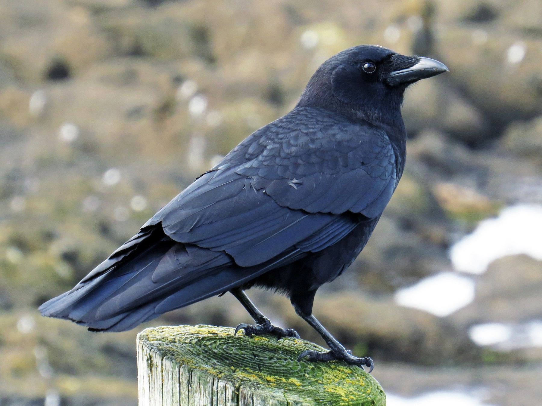<img src='https://test.cdn.download.ams.birds.cornell.edu/api/v1/asset/59858041/1800' width=500 height=300/>\nEntirely black. Large, long-legged, thick-necked bird with heavy, straight bill. In flight, wings are fairly broad and rounded with wingtip feathers spread like fingers. Short tail, squared off at the end. Very social, sometimes forming noisy flocks in the thousands. Aggressive, often chase away hawks and owls. Common in fields, woods, and cities. Thrives around people.","execution_count":null},{"metadata":{"_kg_hide-input":true,"trusted":true},"cell_type":"code","source":"plot_wav('Alder Flycatcher')","execution_count":null,"outputs":[]},{"metadata":{},"cell_type":"markdown","source":"## House Wren\n<img src='https://test.cdn.download.ams.birds.cornell.edu/api/v1/asset/59860711/1800' width=500 height=300/>\nAt home in suburbs, parks, rural farmland, and other open areas with thick tangles. In the breeding season, it is often singing its effervescent song from the top of a bush or fence post. Plumage doesn't show much contrast: plain brown overall, slightly paler below, with some dark barring on the wings and tail. Lacks white eyebrow. In winter they are more secretive, preferring brushy tangles, thickets, and hedgerows.","execution_count":null},{"metadata":{"_kg_hide-input":true,"trusted":true},"cell_type":"code","source":"plot_wav('House Wren')","execution_count":null,"outputs":[]},{"metadata":{},"cell_type":"markdown","source":"## American Robin\n<img src='https://test.cdn.download.ams.birds.cornell.edu/api/v1/asset/60412911/1800' width=500 height=300/>\nFairly large songbird with round body, long legs, and longish tail. Gray above with warm orange underparts and blackish head. Hops across lawns and stands erect with its bill often tilted upward. In fall and winter, forms large flocks and gathers in trees to roost or eat berries. Common across North America in gardens, parks, yards, golf courses, fields, pastures, and many other wooded habitats.","execution_count":null},{"metadata":{"_kg_hide-input":true,"trusted":true},"cell_type":"code","source":"plot_wav('American Robin')","execution_count":null,"outputs":[]},{"metadata":{},"cell_type":"markdown","source":"## Ovenbird\n<img src='https://test.cdn.download.ams.birds.cornell.edu/api/v1/asset/64439011/1800' width=500 height=300/>\nSecretive warbler that lacks vibrant colors, but compensates with its enormous voice. Olive-brown above with black streaks on white breast and bold white eyering. Orange crown bordered by black on either side. Forages for insects by walking along branches and on the ground. Breeds primarily in areas with extensive forest. Listen for its loud song that builds in volume: \"tea-cher, TEA-cher, TEA-CHER!\" Possible to confuse with thrushes, but smaller, and walks instead of hops. Winters in Central America.","execution_count":null},{"metadata":{"_kg_hide-input":true,"trusted":true},"cell_type":"code","source":"plot_wav('Ovenbird')","execution_count":null,"outputs":[]},{"metadata":{},"cell_type":"markdown","source":"## Northern Flicker\n<img src='https://test.cdn.download.ams.birds.cornell.edu/api/v1/asset/60403261/1800' width=500 height=300/>\nLarge, brown woodpecker with black barring on the back and black spots on the belly. Easily recognized in flight by its bright white rump. Also note large black crescent-shaped mark on breast. Underwings are yellow or red, depending on the subspecies. Generally \"Yellow-shafted\" is found in eastern and northern North America, and \"Red-shafted\" in the West south through Mexico. Often seen feeding on the ground in lawns, where they eat lots of ants and worms. Nests in cavities.","execution_count":null},{"metadata":{"_kg_hide-input":true,"trusted":true},"cell_type":"code","source":"plot_wav('Northern Flicker')","execution_count":null,"outputs":[]},{"metadata":{},"cell_type":"markdown","source":"# Bird Chirp Rating system\nSo the site https://www.xeno-canto.org/ rates the chirp of the bird. On further analysis of the dataset and the site, I found that the birds are rated on a scale of 0-5 with 0 being the least and 5 being the highest rating. In this section, I'll be analysing the ratings and what factors are actually affecting the rating of the bird chirp.","execution_count":null},{"metadata":{},"cell_type":"markdown","source":"## How are the birds rated?\nLet's just see what number of unique birds are assigned to which rating. This can be analysed using a bar plot.","execution_count":null},{"metadata":{"trusted":true,"_kg_hide-input":true},"cell_type":"code","source":"#Common backdrop to be used for all the plots\nPAPER_BGCOLOR='rgb(255,255,255)'\nPLOT_BGCOLOR='rgb(255,255,255)'","execution_count":null,"outputs":[]},{"metadata":{"trusted":true,"_kg_hide-input":true},"cell_type":"code","source":"ratings = df_train.groupby('rating',as_index=False)['title'].count().sort_values('rating')\nfig = go.Figure()\nfig.add_trace(go.Bar(x=ratings['rating'],y=ratings['title'],marker_line_color='black',marker_line_width=1.5,text=ratings['title'],textposition='auto'))\nfig.update_layout(template='seaborn',height=300,title='Ratings count',paper_bgcolor=PAPER_BGCOLOR,plot_bgcolor=PLOT_BGCOLOR,\n                 xaxis=dict(title='Ratings',nticks=20,mirror=True,linewidth=2,linecolor='black'),\n                 yaxis=dict(title='Counts',mirror=True,linewidth=2,linecolor='black',gridcolor='darkgrey'))\nfig.show()","execution_count":null,"outputs":[]},{"metadata":{},"cell_type":"markdown","source":"**Seems like the people really find all the chirps pretty pleasing :P as most of the birds are rated above 3.5.** ","execution_count":null},{"metadata":{"_kg_hide-input":true,"trusted":true},"cell_type":"code","source":"df_train['year'] = df_train['date'].apply(lambda x: int(x.split('-')[0]))\ngroup = df_train.groupby(['year','species'],as_index=False).agg({'rating':'mean','ebird_code':'count'})\\\n    .sort_values(['year','ebird_code'],axis=0)\ngroup = group[group['year']>=1979]\n\ndata = np.array(list(product(group.year.unique().tolist(),group.species.unique().tolist())))\ndf_data = pd.DataFrame(np.vstack(data), columns=['year','species'])\ndf_data['year'] = df_data['year'].astype(int)\ndf_data = pd.merge(df_data,group,on=['year','species'],how='left')\ndf_data.fillna(0,inplace=True)\ndf_data.rename(columns={'ebird_code':'Recordings'},inplace=True)\ndf_data.Recordings = df_data.Recordings.astype(int)\nfig = px.bar(df_data,y='species',x='Recordings',animation_frame='year',orientation='h')\nfig.update_layout(template='seaborn',height=800,width=700,title='Recordings registered per year',\n                  paper_bgcolor=PAPER_BGCOLOR,plot_bgcolor=PLOT_BGCOLOR,\n                 xaxis=dict(range=[0,48],title='Number of Recordings',mirror=True,linewidth=2,linecolor='black',gridcolor='darkgrey'),\n                 yaxis=dict(title='Bird Species',mirror=True,linewidth=2,linecolor='black'))\nfig.show()","execution_count":null,"outputs":[]},{"metadata":{},"cell_type":"markdown","source":"## What really affects these ratings?\nI have done an extensive analysis of the rating using the following features:-\n- Number of Recordists\n- Number of Countries where the bird is found\n- Mean Duration of the chirp in seconds\n- Mean Elevation of the bird in meters\n\n>In the dashboard below the X-axis of all the scatter plots shows the ratings scale.","execution_count":null},{"metadata":{"trusted":true,"_kg_hide-input":true},"cell_type":"code","source":"ratings_species = df_train.groupby('species',as_index=False)\\\n    .agg({'rating':'mean','country':'nunique','author':'nunique','duration':'mean','elevation':'mean'})\nratings_species['rating']=np.round(ratings_species['rating'],2)\nratings_species['duration']=np.round(ratings_species['duration'],2)\nratings_species['elevation']=np.round(ratings_species['elevation'],2)\nratings_species.sort_values('rating',ascending=False,inplace=True)","execution_count":null,"outputs":[]},{"metadata":{"trusted":true,"_kg_hide-input":true},"cell_type":"code","source":"fig = make_subplots(rows=3,cols=2,specs=[[{'type':'table','colspan':2},None],[{},{}],[{},{}]],\n                   vertical_spacing=0.03,horizontal_spacing=0.03)\nfig.add_trace(go.Table(\n        columnorder=[1,2,3,4,5,6],\n        columnwidth=[170,60,130,90,130,120],\n        header=dict(\n            values=[\"<b>Species</b>\", \"<b>Mean Rating</b>\", \"<b>No. of Countries</b><br>where bird is found\",\n                    \"<b>No. of Recordists</b>\",'<b>Mean Duration</b><br>of chirp in seconds',\n                   \"<b>Mean Elevation</b><br>in meters\"],\n            line_color='darkslategray',\n            fill_color='royalblue',\n            font=dict(color='white', size=10),\n            align=['center']\n        ),\n        cells=dict(\n            values=[ratings_species[k].tolist() for k in ratings_species.columns],\n            align = \"center\",\n            line_color='darkslategray',\n            fill=dict(color=['paleturquoise', 'white']))\n    ),1,1)\nfig.add_trace(go.Scatter(name='Author',x=ratings_species.rating,y=ratings_species.author,mode='markers',\n                        marker_size=10,marker_line_width=1,\n                        text=ratings_species['species'],\n                        textposition='bottom center'),2,1)\nfig.add_trace(go.Scatter(name='Duration',x=ratings_species.rating,y=ratings_species.duration,mode='markers',\n                        marker_size=10,marker_line_width=1,\n                        text=ratings_species['species'],\n                        textposition='bottom center'),2,2)\nfig.add_trace(go.Scatter(name='Country',x=ratings_species.rating,y=ratings_species.country,mode='markers',\n                        marker_size=10,marker_line_width=1,\n                        text=ratings_species['species'],\n                        textposition='bottom center'),3,1)\nfig.add_trace(go.Scatter(name='Elevation',x=ratings_species.rating,y=ratings_species.elevation,mode='markers',\n                        marker_size=10,marker_line_width=1,\n                        text=ratings_species['species'],\n                        textposition='bottom center'),3,2)\n\nfig.update_xaxes(linecolor='black',linewidth=2,showline=True,\n                 showgrid=False,mirror=True,ticks='inside',tickfont=dict(size=10),row=2,col=1)\nfig.update_xaxes(linecolor='black',linewidth=2,showline=True,\n                 showgrid=False,mirror=True,ticks='inside',tickfont=dict(size=10),row=2,col=2)\nfig.update_xaxes(linecolor='black',linewidth=2,showline=True,\n                 showgrid=False,mirror=True,ticks='inside',tickfont=dict(size=10),row=3,col=1)\nfig.update_xaxes(linecolor='black',linewidth=2,showline=True,\n                 showgrid=False,mirror=True,ticks='inside',tickfont=dict(size=10),row=3,col=2)\n\nfig.update_yaxes(title_text='No. of Recordists',linecolor='black',linewidth=2,showline=True,\n                 showgrid=False,mirror=True,ticks='inside',tickfont=dict(size=10),row=2,col=1)\nfig.update_yaxes(title_text='Mean Duration',linecolor='black',linewidth=2,showline=True,side='right',\n                 showgrid=False,mirror=True,ticks='inside',tickfont=dict(size=10),row=2,col=2)\nfig.update_yaxes(title_text='No. of Countries',linecolor='black',linewidth=2,showline=True,\n                 showgrid=False,mirror=True,ticks='inside',tickfont=dict(size=10),row=3,col=1)\nfig.update_yaxes(title_text='Mean Elevation',linecolor='black',linewidth=2,showline=True,side='right',\n                 showgrid=False,mirror=True,ticks='inside',tickfont=dict(size=10),row=3,col=2)\n\nfig.update_layout(template='seaborn',width=700,height=800,title='Bird Chirp Rating Analysis',\n                  showlegend=False,plot_bgcolor=PLOT_BGCOLOR,paper_bgcolor=PAPER_BGCOLOR)\nfig.show()                                            ","execution_count":null,"outputs":[]},{"metadata":{"trusted":true},"cell_type":"code","source":"for graph in fig.data:\n    graph_type = type(graph).__name__\n    if graph_type == 'Bar' or graph_type == 'Scatter':\n        print(graph.marker)\n    ","execution_count":null,"outputs":[]},{"metadata":{},"cell_type":"markdown","source":"**Looks like a positive correlation between all the features and rating.**","execution_count":null},{"metadata":{},"cell_type":"markdown","source":"# Bird Chirp Spatial Analysis\nIn this section, I'll be doing a spatial analysis of the bird chirp recordings. I'll be answering the questions such as:\n- `Which countries had the most number of recordings?`\n- `Which countries produced the best recordings?`\n- `Was the bird seen or not?`\n- `Where the recordings were made?`","execution_count":null},{"metadata":{},"cell_type":"markdown","source":"## Country wise Analysis\nHere, I'll be answering the first three questions using a bar plot. Below is some info about the plot:-\n- The size of the bar represents the number of recordings for a particular country.\n- The colour of the bar represents if the bird was seen or not while recording. Green stands for 'yes' while Red stands for 'no'.\n- The text represents the average rating for the country for both the cases: bird seen or not. It's on a scale of 0-5 with 0 being the lowest and 5 being the highest.\n- Just hover along the y-axis to know all the information about a particular country.\n- I will be represting the Top 50 countries in terms of number of recordings. In total there are 95 distinct countries where the recordings have been done.","execution_count":null},{"metadata":{"_kg_hide-input":true,"trusted":true},"cell_type":"code","source":"countries = df_train.groupby(['country','bird_seen'],as_index=False).agg({'title':'count','rating':'mean'})\\\n    .sort_values('title',ascending=False).reset_index()\ncountries = countries.loc[:50,:]\nseen_color = {'yes':'rgb(93, 217, 93)','no':'rgb(239, 58, 56)'}\nfig = go.Figure()\nfor seen in ['yes','no']:\n    fig.add_trace(go.Bar(name=seen,y=countries[countries['bird_seen']==seen]['country'],\n                         x=countries[countries['bird_seen']==seen]['title'],orientation='h',\n                         marker_line_color='black',marker_line_width=1.5,\n                         text=np.round(countries[countries['bird_seen']==seen]['rating'],2),textposition='outside',\n                         marker_color=seen_color[seen]))\nfig.update_layout(height=800,template='seaborn',paper_bgcolor=PAPER_BGCOLOR,plot_bgcolor=PLOT_BGCOLOR,barmode='stack',\n                  hovermode='y unified',width=700,\n                 xaxis=dict(title='Number of Recordings',type='log',mirror='allticks',linewidth=2,linecolor='black',\n                            showgrid=True,gridcolor='darkgray'),\n                 yaxis=dict(mirror=True,linewidth=2,linecolor='black',tickfont=dict(size=8)),\n                 legend=dict(title='<b>Was the bird seen?</b>',x=0.71,y=0.95,bgcolor='rgba(255, 255, 255, 0)',\n                             bordercolor='rgba(255, 255, 255, 0)'),\n                 title='<b>Number of Recordings per Country [Top 50]</b><br>(Along with average ratings)')\nfig.show()","execution_count":null,"outputs":[]},{"metadata":{},"cell_type":"markdown","source":"**Analysis from the plot above:-**\n- Most number of recordings have come from USA with Canada being a far second having less than 1/5th recordings than that of USA's.\n- In majority of cases the bird is seen while recording. \n- Iceland has the worst average rating of 1.2 from 103 recordings. Bird was seen in all the recordings.\n- Slovakia has the best average rating of 4.97 from 15 records. Bird was seen in all the recordings.","execution_count":null},{"metadata":{},"cell_type":"markdown","source":"## Where the recordings were made?\nSince, I have latitude and longitude of the location where recordings were made, I'll be plotting the exact locations on the map where the recordings were made.","execution_count":null},{"metadata":{"_kg_hide-input":true,"trusted":true},"cell_type":"code","source":"from kaggle_secrets import UserSecretsClient\nuser_secrets = UserSecretsClient()\nsecret_value_0 = user_secrets.get_secret(\"gmaps\")\nsecret_value_1 = user_secrets.get_secret(\"mapboxtoken\")\ndf_train.latitude = df_train.latitude.str.replace('Not specified','nan').astype(np.float16)\ndf_train.longitude = df_train.longitude.str.replace('Not specified','nan').astype(np.float16)","execution_count":null,"outputs":[]},{"metadata":{"trusted":true,"_kg_hide-input":true},"cell_type":"code","source":"px.set_mapbox_access_token(secret_value_1)\nfig = px.scatter_mapbox(df_train,\n                lat='latitude',\n                lon='longitude',\n                size='duration',\n                color='rating',\n                hover_name='species',\n                hover_data=['duration','country','elevation'],\n                color_continuous_scale=px.colors.sequential.Viridis,\n                mapbox_style='open-street-map',\n                zoom=0.5)\nfig.update_geos(fitbounds=\"locations\", visible=True)\nfig.update_geos(projection_type=\"mercator\")\nfig.update_layout(height=500,width=700,margin={\"r\":0,\"t\":50,\"l\":0,\"b\":0})\nfig.update_layout(title='<b>Recording Locations</b>',template='seaborn',\n                  hoverlabel=dict(bgcolor=\"white\", font_size=16, font_family=\"Rockwell\"))\nfig.show()","execution_count":null,"outputs":[]},{"metadata":{},"cell_type":"markdown","source":"**As seen above, most of the recordings were made in North America.**","execution_count":null},{"metadata":{},"cell_type":"markdown","source":"# Recordist Analysis\nNow lets analyse the recordists. A recordist is the one who records the bird chirp. In this dataset we have two columns: `author` & `recordist`, but they are actually the same. Therefore, the person recording and posting the chird online is the same.\n\nIn the below plot I'll be using a table to show details about all the recordists and a bar plot showing the top 30 recordists. I'm not fetching the top 30 recordists by just sorting on the basis of their ratings because a recordist just having a single recording with rating 5 can look better than a recordist with 100 recording having 99 5 ratings and 1 recording with 4 rating. So, to avoid this bias I'll be taking number of countries and species covered by the recordist into consideration along with the average rating. Below is the image of the formula used by me:-\n\n**score = 0.5x(Number of Species Covered) + 0.3x(Number of Countries covered) + 0.2x(Average rating)**\n\n> Please note: All these values are normalized.\n\nSo, the top 30 recordists will be evaluated on the basis of this score. I believe a recordist who have covered a large number of species is better than those who haven't covered many. So, the weightage given species is 50%. Countries and rating have 30% and 20% weightage respectively.","execution_count":null},{"metadata":{"trusted":true,"_kg_hide-input":true},"cell_type":"code","source":"def normalize(x):\n    xmin = x.min()\n    xmax = x.max()\n    return (x-xmin)/(xmax-xmin)\n\nrecordists = df_train.groupby('author',as_index=False).agg({'rating':'mean','species':'nunique','country':'nunique'})\\\n.sort_values(['species','rating'],ascending=False)\nrecordists['rating'] = np.round(recordists['rating'],2)\nrecordists['rating_norm'] = normalize(recordists['rating'])\nrecordists['species_norm'] = normalize(recordists['species'])\nrecordists['country_norm'] = normalize(recordists['country'])\nrecordists['total'] = recordists['species_norm']*0.5 + recordists['country_norm']*0.3 + recordists['rating_norm']*0.2\nrecordists.drop(['rating_norm','species_norm','country_norm'],axis=1,inplace=True)\n\nfig = make_subplots(rows=2,cols=1,specs=[[{'type':'table','rowspan':1}],[{'rowspan':1}]],\n                   vertical_spacing=0.03,horizontal_spacing=0.03,shared_xaxes=True)\nfig.add_trace(go.Table(\n        columnorder=[1,2,3,4],\n        columnwidth=[250,150,150,150],\n        header=dict(\n            values=[\"<b>Recordist</b>\", \"<b>Mean Rating</b>\", \"<b>Species Covered</b>\",\n                    \"<b>Countries Covered</b>\"],\n            line_color='darkslategray',\n            fill_color='royalblue',\n            font=dict(color='white', size=12),\n            align=['center']\n        ),\n        cells=dict(\n            values=[recordists[k].tolist() for k in recordists.columns[:-1]],\n            align = \"center\",\n            line_color='darkslategray',\n            fill=dict(color=['paleturquoise', 'white']))\n    ),1,1)\n\nrec = recordists.nlargest(30,'total')\nfig.add_trace(go.Bar(name='Species',x=rec.author,y=rec.species,\n                    marker_line_width=1.5,\n                    marker_line_color='black',\n                    marker_color='#F1EA49'),2,1)\nfig.add_trace(go.Bar(name='Countries',x=rec.author,y=rec.country,\n                    marker_line_width=1.5,\n                    marker_line_color='black',\n                    marker_color='#3893D2',\n                    text=rec.rating,\n                    textposition='outside'),2,1)\nfig.update_xaxes(linecolor='black',linewidth=2,showline=True,\n                 showgrid=False,mirror=True,ticks='outside',tickfont=dict(size=10),row=2,col=1)\nfig.update_yaxes(title='Species + Countries covered',linecolor='black',linewidth=2,showline=True,\n                 showgrid=False,mirror=True,ticks='outside',tickfont=dict(size=10),row=2,col=1)\nfig.update_layout(template='seaborn',width=700,height=800,title='Recordist Analysis',\n                  legend=dict(title='<b>   Top 30<br>Recordists</b>',x=0.1,y=0.49,bgcolor='rgba(255, 255, 255, 0)',\n                             bordercolor='rgba(255, 255, 255, 0)',orientation='h'),\n                  plot_bgcolor=PLOT_BGCOLOR,paper_bgcolor=PAPER_BGCOLOR,barmode='stack',\n                 hovermode='x unified')\nfig.show()                                            ","execution_count":null,"outputs":[]},{"metadata":{},"cell_type":"markdown","source":"**So, as per my rating scale Mike Nelson is the top Recordist as he has covered the right mix of species and countries. Although, his recordings have an average rating of 3.95 as can be seen from the plot.**","execution_count":null},{"metadata":{"trusted":true,"_kg_hide-input":true,"_kg_hide-output":true},"cell_type":"code","source":"\"\"\"Covert mp3 to wav format\"\"\"\n# path = '/kaggle/input/birdsong-recognition/train_audio/'\n# out_dir = '/kaggle/working/train_audio_wav'\n# if not os.path.exists(out_dir):\n#     os.makedirs(out_dir)\n# for i in range(df_train.shape[0]):\n#     src = os.path.join(path,df_train.loc[i,'ebird_code'],df_train.loc[i,'filename'])\n#     dst = os.path.join(out_dir,df_train.loc[i,'ebird_code'])\n#     if not os.path.exists(dst):\n#         os.makedirs(dst)\n#     sound = AudioSegment.from_mp3(src)\n#     os.chdir(dst)\n#     sound.export(df_train.loc[i,'filename'].split('.')[0]+'.wav', format='wav')    ","execution_count":null,"outputs":[]},{"metadata":{},"cell_type":"markdown","source":"### Just an initial commit. Lot more of EDA to come. Do leave an upvote if you liked my work. It encourages me to produce more quality content.","execution_count":null}],"metadata":{"kernelspec":{"language":"python","display_name":"Python 3","name":"python3"},"language_info":{"pygments_lexer":"ipython3","nbconvert_exporter":"python","version":"3.6.4","file_extension":".py","codemirror_mode":{"name":"ipython","version":3},"name":"python","mimetype":"text/x-python"}},"nbformat":4,"nbformat_minor":4}