.png?generation=1749292477050741&alt=media\")
\n\nI know that Kagglers are aware of what’s happening in Ukraine, and you’re here to take a look at my solution, but let me share a small glimpse from the competition’s deadline day that reflects our current reality: I had to make my final submissions from a shelter while we had a stable connection, as Ukraine was under another devastating attack with many civilian casualties, some of them from my neighborhood. \n I would like to thank the Armed Forces of Ukraine, Security Service of Ukraine, Defence Intelligence of Ukraine, and the State Emergency Service of Ukraine for providing safety and security to participate in this great competition, complete this work, and help science, technology, and business not to stop but to move forward.
\n
The Insecta group included labels at the family level, such as Cicadidae, Gryllidae, and Tettigoniidae, while the rest of the Insecta labels were species from the Tettigoniidae family. But the following experiments showed that the family-level labels were probably related to the specific species or at least to a narrow set of species that inhabit the Middle Magdalena Valley:
\nFrom the start, I came to the thought that the presence of Amphibia and Insecta groups would make models favor longer input durations over shorter ones, since the long duration and repetitiveness of their calls are distinctive features for species from these groups.\nTo find the most optimal duration, I conducted multiple experiments with different durations and figured that 20-second chunks work best for me, and any longer duration did not improve results but took more time to infer, so I continued with that chunk duration. \nHere are the Public scores that I obtained by experimenting with different durations while training(supervised with train data only) an ensemble of 5 SED efficientnetb0 models and adjusting proportionally spectrogram hop length(more detailed information on the models and inference is provided in the next sections):
\n| Chunk duration | \nPublic LB | \n
|---|---|
| 5 sec | \n0.842 | \n
| 10 sec | \n0.864 | \n
| 15 sec | \n0.87 | \n
| 20 sec | \n0.872 | \n
| 30 sec | \n0.872 | \n
Across different training stages, I used various CNNs, gradually incorporating more complex models at each stage. All models included the SED head (adaptation from the 4th place 2021 ), which consistently provided a significant boost over other head variations.
\nAs it turned out, the Hosts were absolutely honest with us(did not have any doubt), and most Public results correlated pretty well with the private LB.
\nI noticed that the choice of loss got a lot of attention in the discussions. So I conducted some experiments and found that both CE and BCE/Focal losses could give me similar results when the learning rate and the number of epochs were well-tuned. However, CE gave me a bit better results, so I settled on it.\nI connect better results with CE (I might be wrong) with the following interconnected assumptions:
\nAlso, I didn’t normalize sample labels to sum to one, motivated by the idea that more difficult samples (those with more positive labels) should have a greater impact on the loss.
\n.png?generation=1749300190075357&alt=media\")
I am showing my inference flow first to give more context before going to the next sections, where I explain how I used pseudo-labels, which were generated with that inference. I hope my diagram does not look too overloaded. \nThe core idea was to fully leverage all framewise predictions produced by the SED head by averaging the overlapping framewise predictions from neighboring audio chunks, rather than taking max only from the central 5 sec and throwing away precious predictions.
\nAfter hitting the ceiling with the supervised approach, it became clear that further improvements would come with the usage of the unlabeled soundscapes. \nI pseudo-labeled the unlabeled data using the best LB ensemble from the 1 stage with the described above inference flow, and began experimenting with the ways to incorporate pseudo-labeled data in the training. \nInitial attempts to concatenate the pseudo-labeled data into training batches separately didn’t succeed.
\nThen I tried mixing up the pseudo-labeled raw data with the training raw data, following the approach from the 2nd place solution 2024. At first, it didn’t work because I had set the Beta distribution’s parameters to be too low(used to sample blending weights). But after switching to a constant blending weight of 0.5(Beta’s parameters = inf), the magic started to happen, and the LB score began to rise. I suspect that is related to the fact that blending weights far from 0.5 sometimes suppress the meaningful signals, especially when mixing relatively clear train data with much noisier train soundscapes.
\nReading the paper on the Noisy Student approach [1], I found certain similarities with the self-training approach I was using. \nSo, I started experimenting with the techniques that showed a positive impact on self-training in the mentioned paper and found that adding Stochastic Depth [3] (i.e., dropout applied to the entire residual blocks) worked for me as well.
\ndrop_path_rate = 0.15 (which turned out to be optimal for all the models I trained), I consistently saw a boost in the LB score, up to 0.005 for some models. \n\nAfter reading [1], I finally understood why mixup works while simple concatenation doesn’t. Since it closely matched my approach, I considered it a form of Noisy Student self-training and named my solution accordingly.\n Putting simply - showing to the model the same input and asking for the same output does not teach the student anything new, so in the best case it converges to the same results, in the worst case it accumulates error and the LB score drops (what I experienced). But when we inject noise(augmentations like mixup, drop paths) and ask to provide the same output as for the clean input, it starts learning more robust features instead of accumulating error. \n I imagined the following scenario: we have a pseudo-labeled sample where A is the true label, and B is the negative one. The teacher model predicts A ≈ 1 and B ≈ 0, but not exactly zero. If we repeatedly train on this same input, the model may start learning irrelevant features associated with B, simply because its score isn’t exactly zero. It may also overfit to some noise because of thinking that it is related to A. At the same time, it doesn’t offer anything new beyond what the teacher model has already seen and learned, so it doesn’t lead to any improvement.\n However, if we augment that sample, the student model must work harder to understand why the teacher gave a high score to A(an unaugmented input for the teacher). As a result, through this noisy student training, we force the model to focus on the most consistent, generalizable features relevant to A rather than memorizing noise associated with A and B.\n Also, Noisy Student methodology involves including labeled samples in training (as I did), whose signals help guide the model toward better optima, especially during the early epochs.\n And MixUps with pseudo-labeled data serve as a great augmentation for labeled samples, providing target domain backgrounds with soft-labels for possible species in that background.
\n
| Ratio of mixed samples | \nPublic LB | \n
|---|---|
| 0 (labeled training data only) | \n0.872 | \n
| 0.25 | \n0.883 | \n
| 0.5 | \n0.887 | \n
| 0.75 | \n0.89 | \n
| 1.0 | \n0.898 | \n
Inspired by the 2nd place solution 2024 and papers on self-training [1, 2], I tried to pseudo-label the unlabeled soundscapes again, using models that were already trained on the pseudo-labels from the previous iteration. However, this approach didn’t work out of the box, and I spent some time investigating why until I found the correct preprocessing of the pseudo-labels that allowed me to keep training models on the next pseudo-labeling iterations.
\nThe reason the models failed to converge in later iterations was that the pseudo-labels had become too noisy, obscuring any meaningful signal. \nHere is the method that worked best for me and allowed me to move forward:
\nIn the image below, you can see that the power transform is a real power in the fight against label noise. After the transformation, labels become much cleaner, and only initially confident labels survive, having still pronounced values to train models.\n
Knowing how to train a multi-iterative noisy student, I ran 4 iterations, adjusting the pseudo-label power at each stage by validating results on the LB and consistently got the LB boost.\nThat self-training magic stopped working on the 5th pseudo-labeling iteration. I could not achieve any further improvement, so I stopped with the attempts to make new iterations work.
\n| Iteration | \nPower value | \nPublic LB | \n
|---|---|---|
| 1 | \n1 | \n0.909 | \n
| 2 | \n1 / 0.65 | \n0.918 | \n
| 3 | \n1 / 0.55 | \n0.927 | \n
| 4 | \n1 / 0.6 | \n0.93 | \n
Knowing that species groups like Amphibia and Insecta are very underrepresented, and that Xeno-Canto provides data for multiple species from those groups that are not present in the train, I decided to try training a separate model that would see samples only from those groups, with a much higher diversity of species. The motivation was that the model would learn more representative features relevant to those groups, which would be a great supplement to the models that are trained only on a restricted number of samples/species from the training data.
\nAfter finding the optimal working parameters, I achieved a 0.002–0.003 LB boost.
\nI found that ensembling models from different training stages was beneficial not only for slightly improving the LB score, but also for giving me a little confidence that my solution is not overfitted by doing more and more self-training iterations.
\nThe final ensemble consisted of the following 7 models trained on the specific data and different self-training iterations:
\nIn my best solution, I tweaked the ensembling weights a bit, giving to efficientnetb3 and ecanfnetl0 slightly higher weights since they performed better as single models. However, the best private submission, with a score of 0.935, was achieved when I assigned equal weights to all models.
\nI believe that the ensembling of multi-stage models, diverse backbone architectures, and the dedicated model to certain species groups were crucial parts of my solution to withstanding the shake-up.\nAs a result, my best public LB score dropped only slightly on the private LB from 0.933 to 0.930.
\nI apologize that my write-up turned out to be a bit long. I did not want to skip anything important. \nMy Google Sheet accumulated during the competition over 320+ rows of ideas to check (95% of which were eventually marked red). So I decided not to include the What did not work block, otherwise it would significantly increase the length of the already long write-up.\nPlease feel free to ask me any questions about my solution in the comments. I will do my best to answer them.
I also want to thank all the participants of the previous BirdCLEF iterations who shared their ideas.\nWithout your brilliant ideas, I would not have been able to achieve that result.
\nSpecial thanks to the organizers, hosts, and everyone involved in conducting BirdCLEF. It is very appreciated that you put so much effort into conducting BirdCLEF each year, that you constantly stay in touch, and make each new iteration special(which is reflected in this year's number of participants).
\n[1] Self-training with Noisy Student improves ImageNet classification\n[2] Design Choices for Enhancing Noisy Student Self-Training\n[3] Deep Networks with Stochastic Depth
\nInference notebook: https://www.kaggle.com/code/nikitababich/birdclef2025-1st-place-inference\nDatasets: Extra Xeno-Canto data used in the solution
", "messages": [ { "id": 3219545, "postDate": "2025-06-07T23:20:45.843Z", "content": "\n\nI know that Kagglers are aware of what’s happening in Ukraine, and you’re here to take a look at my solution, but let me share a small glimpse from the competition’s deadline day that reflects our current reality: I had to make my final submissions from a shelter while we had a stable connection, as Ukraine was under another devastating attack with many civilian casualties, some of them from my neighborhood. \n I would like to thank the Armed Forces of Ukraine, Security Service of Ukraine, Defence Intelligence of Ukraine, and the State Emergency Service of Ukraine for providing safety and security to participate in this great competition, complete this work, and help science, technology, and business not to stop but to move forward.
\n
The Insecta group included labels at the family level, such as Cicadidae, Gryllidae, and Tettigoniidae, while the rest of the Insecta labels were species from the Tettigoniidae family. But the following experiments showed that the family-level labels were probably related to the specific species or at least to a narrow set of species that inhabit the Middle Magdalena Valley:
\nFrom the start, I came to the thought that the presence of Amphibia and Insecta groups would make models favor longer input durations over shorter ones, since the long duration and repetitiveness of their calls are distinctive features for species from these groups.\nTo find the most optimal duration, I conducted multiple experiments with different durations and figured that 20-second chunks work best for me, and any longer duration did not improve results but took more time to infer, so I continued with that chunk duration. \nHere are the Public scores that I obtained by experimenting with different durations while training(supervised with train data only) an ensemble of 5 SED efficientnetb0 models and adjusting proportionally spectrogram hop length(more detailed information on the models and inference is provided in the next sections):
\n| Chunk duration | \nPublic LB | \n
|---|---|
| 5 sec | \n0.842 | \n
| 10 sec | \n0.864 | \n
| 15 sec | \n0.87 | \n
| 20 sec | \n0.872 | \n
| 30 sec | \n0.872 | \n
Across different training stages, I used various CNNs, gradually incorporating more complex models at each stage. All models included the SED head (adaptation from the 4th place 2021 ), which consistently provided a significant boost over other head variations.
\nAs it turned out, the Hosts were absolutely honest with us(did not have any doubt), and most Public results correlated pretty well with the private LB.
\nI noticed that the choice of loss got a lot of attention in the discussions. So I conducted some experiments and found that both CE and BCE/Focal losses could give me similar results when the learning rate and the number of epochs were well-tuned. However, CE gave me a bit better results, so I settled on it.\nI connect better results with CE (I might be wrong) with the following interconnected assumptions:
\nAlso, I didn’t normalize sample labels to sum to one, motivated by the idea that more difficult samples (those with more positive labels) should have a greater impact on the loss.
\n
I am showing my inference flow first to give more context before going to the next sections, where I explain how I used pseudo-labels, which were generated with that inference. I hope my diagram does not look too overloaded. \nThe core idea was to fully leverage all framewise predictions produced by the SED head by averaging the overlapping framewise predictions from neighboring audio chunks, rather than taking max only from the central 5 sec and throwing away precious predictions.
\nAfter hitting the ceiling with the supervised approach, it became clear that further improvements would come with the usage of the unlabeled soundscapes. \nI pseudo-labeled the unlabeled data using the best LB ensemble from the 1 stage with the described above inference flow, and began experimenting with the ways to incorporate pseudo-labeled data in the training. \nInitial attempts to concatenate the pseudo-labeled data into training batches separately didn’t succeed.
\nThen I tried mixing up the pseudo-labeled raw data with the training raw data, following the approach from the 2nd place solution 2024. At first, it didn’t work because I had set the Beta distribution’s parameters to be too low(used to sample blending weights). But after switching to a constant blending weight of 0.5(Beta’s parameters = inf), the magic started to happen, and the LB score began to rise. I suspect that is related to the fact that blending weights far from 0.5 sometimes suppress the meaningful signals, especially when mixing relatively clear train data with much noisier train soundscapes.
\nReading the paper on the Noisy Student approach [1], I found certain similarities with the self-training approach I was using. \nSo, I started experimenting with the techniques that showed a positive impact on self-training in the mentioned paper and found that adding Stochastic Depth [3] (i.e., dropout applied to the entire residual blocks) worked for me as well.
\ndrop_path_rate = 0.15 (which turned out to be optimal for all the models I trained), I consistently saw a boost in the LB score, up to 0.005 for some models. \n\nAfter reading [1], I finally understood why mixup works while simple concatenation doesn’t. Since it closely matched my approach, I considered it a form of Noisy Student self-training and named my solution accordingly.\n Putting simply - showing to the model the same input and asking for the same output does not teach the student anything new, so in the best case it converges to the same results, in the worst case it accumulates error and the LB score drops (what I experienced). But when we inject noise(augmentations like mixup, drop paths) and ask to provide the same output as for the clean input, it starts learning more robust features instead of accumulating error. \n I imagined the following scenario: we have a pseudo-labeled sample where A is the true label, and B is the negative one. The teacher model predicts A ≈ 1 and B ≈ 0, but not exactly zero. If we repeatedly train on this same input, the model may start learning irrelevant features associated with B, simply because its score isn’t exactly zero. It may also overfit to some noise because of thinking that it is related to A. At the same time, it doesn’t offer anything new beyond what the teacher model has already seen and learned, so it doesn’t lead to any improvement.\n However, if we augment that sample, the student model must work harder to understand why the teacher gave a high score to A(an unaugmented input for the teacher). As a result, through this noisy student training, we force the model to focus on the most consistent, generalizable features relevant to A rather than memorizing noise associated with A and B.\n Also, Noisy Student methodology involves including labeled samples in training (as I did), whose signals help guide the model toward better optima, especially during the early epochs.\n And MixUps with pseudo-labeled data serve as a great augmentation for labeled samples, providing target domain backgrounds with soft-labels for possible species in that background.
\n
| Ratio of mixed samples | \nPublic LB | \n
|---|---|
| 0 (labeled training data only) | \n0.872 | \n
| 0.25 | \n0.883 | \n
| 0.5 | \n0.887 | \n
| 0.75 | \n0.89 | \n
| 1.0 | \n0.898 | \n
Inspired by the 2nd place solution 2024 and papers on self-training [1, 2], I tried to pseudo-label the unlabeled soundscapes again, using models that were already trained on the pseudo-labels from the previous iteration. However, this approach didn’t work out of the box, and I spent some time investigating why until I found the correct preprocessing of the pseudo-labels that allowed me to keep training models on the next pseudo-labeling iterations.
\nThe reason the models failed to converge in later iterations was that the pseudo-labels had become too noisy, obscuring any meaningful signal. \nHere is the method that worked best for me and allowed me to move forward:
\nIn the image below, you can see that the power transform is a real power in the fight against label noise. After the transformation, labels become much cleaner, and only initially confident labels survive, having still pronounced values to train models.\n
Knowing how to train a multi-iterative noisy student, I ran 4 iterations, adjusting the pseudo-label power at each stage by validating results on the LB and consistently got the LB boost.\nThat self-training magic stopped working on the 5th pseudo-labeling iteration. I could not achieve any further improvement, so I stopped with the attempts to make new iterations work.
\n| Iteration | \nPower value | \nPublic LB | \n
|---|---|---|
| 1 | \n1 | \n0.909 | \n
| 2 | \n1 / 0.65 | \n0.918 | \n
| 3 | \n1 / 0.55 | \n0.927 | \n
| 4 | \n1 / 0.6 | \n0.93 | \n
Knowing that species groups like Amphibia and Insecta are very underrepresented, and that Xeno-Canto provides data for multiple species from those groups that are not present in the train, I decided to try training a separate model that would see samples only from those groups, with a much higher diversity of species. The motivation was that the model would learn more representative features relevant to those groups, which would be a great supplement to the models that are trained only on a restricted number of samples/species from the training data.
\nAfter finding the optimal working parameters, I achieved a 0.002–0.003 LB boost.
\nI found that ensembling models from different training stages was beneficial not only for slightly improving the LB score, but also for giving me a little confidence that my solution is not overfitted by doing more and more self-training iterations.
\nThe final ensemble consisted of the following 7 models trained on the specific data and different self-training iterations:
\nIn my best solution, I tweaked the ensembling weights a bit, giving to efficientnetb3 and ecanfnetl0 slightly higher weights since they performed better as single models. However, the best private submission, with a score of 0.935, was achieved when I assigned equal weights to all models.
\nI believe that the ensembling of multi-stage models, diverse backbone architectures, and the dedicated model to certain species groups were crucial parts of my solution to withstanding the shake-up.\nAs a result, my best public LB score dropped only slightly on the private LB from 0.933 to 0.930.
\nI apologize that my write-up turned out to be a bit long. I did not want to skip anything important. \nMy Google Sheet accumulated during the competition over 320+ rows of ideas to check (95% of which were eventually marked red). So I decided not to include the What did not work block, otherwise it would significantly increase the length of the already long write-up.\nPlease feel free to ask me any questions about my solution in the comments. I will do my best to answer them.
I also want to thank all the participants of the previous BirdCLEF iterations who shared their ideas.\nWithout your brilliant ideas, I would not have been able to achieve that result.
\nSpecial thanks to the organizers, hosts, and everyone involved in conducting BirdCLEF. It is very appreciated that you put so much effort into conducting BirdCLEF each year, that you constantly stay in touch, and make each new iteration special(which is reflected in this year's number of participants).
\n[1] Self-training with Noisy Student improves ImageNet classification\n[2] Design Choices for Enhancing Noisy Student Self-Training\n[3] Deep Networks with Stochastic Depth
\nInference notebook: https://www.kaggle.com/code/nikitababich/birdclef2025-1st-place-inference\nDatasets: Extra Xeno-Canto data used in the solution
", "rawMarkdown": ">I know that Kagglers are aware of what’s happening in Ukraine, and you’re here to take a look at my solution, but let me share a small glimpse from the competition’s deadline day that reflects our current reality: I had to make my final submissions from a shelter while we had a stable connection, as Ukraine was under another devastating attack with many civilian casualties, some of them from my neighborhood. \n*I would like to thank the Armed Forces of Ukraine, Security Service of Ukraine, Defence Intelligence of Ukraine, and the State Emergency Service of Ukraine for providing safety and security to participate in this great competition, complete this work, and help science, technology, and business not to stop but to move forward.*\n\n## TLDR\n- SED models on 20-second input chunks.\n- A Multi-Iterative Noisy Student is used as a self-training approach via MixUp between focal training data and pseudo-labeled soundscapes.\n- Power transform applied to pseudo-labels to reduce noise.\n- Pseudo-label sampler assigns weights equal to the sum of the maximum of labels within each soundscape.\n- A separate model for Amphibia and Insecta label groups using extended species data from Xeno-Canto.\n- A final ensemble with models from different training iterations.\n- Inference is performed by averaging overlapping framewise predictions from neighboring chunks, followed by smoothing and delta shift inference.\n\n## Solution Overview\n.png?generation=1749292477050741&alt=media)\n\n### Data\n#### Additional Xeno-Canto Data\n- Target species\n - Num samples: 5489\n - Samples per species groups: Aves(birds)=5480, Amphibia=6, Mammalia=3\n - Max samples per species: 500\n - Comment: It usually worsened results, so only one model saw that data.\n- Extra species \n - Num samples: 17197\n - Samples per species groups: Insecta=16218(544 extra species), Amphibia=979(113 extra species)\n - Max samples per species: 200\n - Additional filters: duration less than 60 sec\n - Comment: This data was used to train a separate dedicated model for the Insecta and Amphibia groups.\n\n#### Interesting note about Insecta\nThe Insecta group included labels at the family level, such as Cicadidae, Gryllidae, and Tettigoniidae, while the rest of the Insecta labels were species from the Tettigoniidae family. But the following experiments showed that the family-level labels were probably related to the specific species or at least to a narrow set of species that inhabit the Middle Magdalena Valley:\n- Including the Tettigoniidae label in secondary labels of species from the Tettigoniidae family worsened results. \n- Including extra Xeno-Canto data for Gryllidae and Tettigoniidae (i.e., family-level labels) in training on target species also worsened results.\n- Using additional Gryllidae and Tettigoniidae samples from Xeno-Canto, assigning them unique new labels based on the species of each sample instead of assigning the family-level labels, and training a dedicated model improved results. It means that Tettigoniidae and Gryllidae target labels are related to the specific species that can be separated from other species within these families that are present as other Insecta target labels or extra species from these families that were downloaded.\n\n####Data preparation\n- 5 folds\n- Each fold includes at least 1 sample for each label\n- 20-second audio chunks normalized by absmax\n- All secondary labels = 1\n\nFrom the start, I came to the thought that the presence of Amphibia and Insecta groups would make models favor longer input durations over shorter ones, since the long duration and repetitiveness of their calls are distinctive features for species from these groups.\nTo find the most optimal duration, I conducted multiple experiments with different durations and figured that 20-second chunks work best for me, and any longer duration did not improve results but took more time to infer, so I continued with that chunk duration. \nHere are the Public scores that I obtained by experimenting with different durations while training(supervised with train data only) an ensemble of 5 SED efficientnetb0 models and adjusting proportionally spectrogram hop length(more detailed information on the models and inference is provided in the next sections):\n| Chunk duration | Public LB |\n| --- | --- |\n|5 sec | 0.842 |\n|10 sec | 0.864 |\n|15 sec | 0.87 |\n|**20 sec** | **0.872** |\n|30 sec | 0.872 |\n\n### Models\n#### Architectures\nAcross different training stages, I used various CNNs, gradually incorporating more complex models at each stage. All models included the SED head (adaptation from [the 4th place 2021](https://www.kaggle.com/competitions/birdclef-2021/discussion/243293) ), which consistently provided a significant boost over other head variations.\n- SED \n- Gem frequency pooling \n- Repeated 3 Mel Spectrograms as input\n- 1 stage backbones: \n - tf_efficientnet_b0.ns_jft_in1k \n - regnety_008.pycls_in1k\n- 1 pseudo-labeling iteration backbones: \n - tf_efficientnet_b0.ns_jft_in1k \n - regnety_008.pycls_in1k\n - tf_efficientnet_b3.ns_jft_in1k \n - regnety_016.tv2_in1k\n- 2-4 pseudo-labeling iteration backbones: \n - tf_efficientnet_b3.ns_jft_in1k \n - tf_efficientnet_b4.ns_jft_in1k \n - regnety_016.tv2_in1k \n - eca_nfnet_l0.ra2_in1k\n- Amphibia/Insecta model backbone: \n - tf_efficientnet_b0.ns_jft_in1k \n\n#### Mel spectrogram parameters\n- 20 sec -> Image size = (3, 224, 512)\n- MelSpectrogram (sample_rate: 32000, mel_bins: 224, fmin: 0, fmax: 16000, n_fft: 4096, hop_size: 1252, top_db=80.0)\n- 0-1 normalization\n\n##### Thoughts on mel parameters tuning\n- Because long input chunks were used, I had to set a larger hop length value, otherwise, inference would take too long, and I wouldn’t have the capacity to prepare a good ensemble. \n- The important thing was setting a larger number of n_mels. I suspect this is because some species (especially from the Amphibia and Insecta groups) have calls within narrow frequency ranges, so showing more mel bands to models was important to distinguish species well.\n\n### Validation\n- I did not find a good CV/ LB correlation, so considering the Host's words that public/private distributions are very similar and the knowledge from last year's solutions, I validated ideas using only the public LB. \n- A single model’s LB score varied a lot for different seeds, so usually I trained the same setup on different folds(2-5, depending on the remaining time that I had) and ensembled them to obtain a more reliable response from the LB.\n\nAs it turned out, the Hosts were absolutely honest with us(did not have any doubt), and most Public results correlated pretty well with the private LB.\n\n### 1 Stage (Supervised Learning)\n#### Training Details \n- Epochs: 15\n- Loss: CrossEntropy\n- LR: 5e-4 - 1e-6(same for all models)\n- Optimizer: AdamW with 1e-4 weight decay\n- Scheduler: CosineAnnealingWarmRestarts with restart after each 5 epochs. Applying warm restarts, I could train longer than with one cycle\n- BS: 64\n- Augmentations: \n - Mixup: p = 0.5, on normalized by absmax raw audio with an equal sampling weight for each species\n- Padding: To keep samples of different lengths overlapping after mixup, the left part of it was filled with 0, so on the right, there is always an overlap that ensures train samples are always actually mixed up\n- Models: efficientnet0, regnety8. An ensemble of small models on the 1st stage gave almost the same results as ensembling deeper ones\n\n#### Loss choice\nI noticed that the choice of loss got a lot of attention in the discussions. So I conducted some experiments and found that both CE and BCE/Focal losses could give me similar results when the learning rate and the number of epochs were well-tuned. However, CE gave me a bit better results, so I settled on it.\nI connect better results with CE (I might be wrong) with the following interconnected assumptions: \n- The magnitude of updates with CE for each label depends on how well the positive labels (probability > 0) are classified. This means that if a rare positive label A gets a low probability, then the negative overrepresented label B(that has a higher probability than other negative labels) is pushed to zero with a stronger update. \n- CE handles imbalanced labels better and avoids overfitting to overrepresented classes by punishing them when Softmax can not give a higher score for A because the overrepresented label B already got too high logits as a result of the previous numerous imbalanced updates when label B was positive.\n\nAlso, I didn’t normalize sample labels to sum to one, motivated by the idea that more difficult samples (those with more positive labels) should have a greater impact on the loss.\n\n### Inference\n.png?generation=1749300190075357&alt=media)\n\nI am showing my inference flow first to give more context before going to the next sections, where I explain how I used pseudo-labels, which were generated with that inference. I hope my diagram does not look too overloaded. \nThe core idea was to fully leverage all framewise predictions produced by the SED head by averaging the overlapping framewise predictions from neighboring audio chunks, rather than taking max only from the central 5 sec and throwing away precious predictions.\n- It can be seen as a 1D analogue of 2D sliding-window segmentation of large images, rather than treating each audio chunk as a completely separate sample. \n- It can be seen as a form of test-time augmentation (TTA) because each framewise prediction is averaged over multiple chunks that present the same time frame to the model with slightly different surrounding context.\n- Consistently boosted my LB score (by 0.002-0.003).\n- Helped to get more generalizable predictions. \n\n#### Other inference/postprocessing tricks \n- Padded the left and right sides of the signal to ensure that the first and last 5-second chunks are centered after splitting. Framewise predictions related to the padding were then removed.\n- Smoothing [0.1, 0.2, 0.4, 0.2, 0.1].\n- Delta shift TTA (from [the 2nd solution 2023](https://www.kaggle.com/competitions/birdclef-2023/discussion/412707)).\n\n### Self-training \nAfter hitting the ceiling with the supervised approach, it became clear that further improvements would come with the usage of the unlabeled soundscapes. \nI pseudo-labeled the unlabeled data using the best LB ensemble from the 1 stage with the described above inference flow, and began experimenting with the ways to incorporate pseudo-labeled data in the training. \nInitial attempts to concatenate the pseudo-labeled data into training batches separately didn’t succeed. \n\n#### MixUps (finally working) \nThen I tried mixing up the pseudo-labeled raw data with the training raw data, following the approach from [the 2nd place solution 2024](https://www.kaggle.com/competitions/birdclef-2024/discussion/512340). At first, it didn’t work because I had set the Beta distribution’s parameters to be too low(used to sample blending weights). But after switching to a constant blending weight of 0.5(Beta’s parameters = inf), the magic started to happen, and the LB score began to rise. I suspect that is related to the fact that blending weights far from 0.5 sometimes suppress the meaningful signals, especially when mixing relatively clear train data with much noisier train soundscapes.\n\n##### Stochastic Depth\nReading the paper on the Noisy Student approach [1], I found certain similarities with the self-training approach I was using. \nSo, I started experimenting with the techniques that showed a positive impact on self-training in the mentioned paper and found that adding Stochastic Depth [3] (i.e., dropout applied to the entire residual blocks) worked for me as well.\n- Applying `drop_path_rate = 0.15` (which turned out to be optimal for all the models I trained), I consistently saw a boost in the LB score, up to 0.005 for some models. \n- Applying Stochastic Depth during supervised training didn’t lead to any improvement, which supports the idea that the current self-training approach is a form of Noisy Student self-training.\n\n#### Why Noisy Student? (my understanding)\n>After reading [1], I finally understood why mixup works while simple concatenation doesn’t. Since it closely matched my approach, I considered it a form of Noisy Student self-training and named my solution accordingly.\nPutting simply - showing to the model the same input and asking for the same output does not teach the student anything new, so in the best case it converges to the same results, in the worst case it accumulates error and the LB score drops (what I experienced). But when we inject noise(augmentations like mixup, drop paths) and ask to provide the same output as for the clean input, it starts learning more robust features instead of accumulating error. \nI imagined the following scenario: we have a pseudo-labeled sample where A is the true label, and B is the negative one. The teacher model predicts A ≈ 1 and B ≈ 0, but not exactly zero. If we repeatedly train on this same input, the model may start learning irrelevant features associated with B, simply because its score isn’t exactly zero. It may also overfit to some noise because of thinking that it is related to A. At the same time, it doesn’t offer anything new beyond what the teacher model has already seen and learned, so it doesn’t lead to any improvement.\nHowever, if we augment that sample, the student model must work harder to understand why the teacher gave a high score to A(an unaugmented input for the teacher). As a result, through this noisy student training, we force the model to focus on the most consistent, generalizable features relevant to A rather than memorizing noise associated with A and B.\nAlso, Noisy Student methodology involves including labeled samples in training (as I did), whose signals help guide the model toward better optima, especially during the early epochs.\nAnd MixUps with pseudo-labeled data serve as a great augmentation for labeled samples, providing target domain backgrounds with soft-labels for possible species in that background.\n\n#### Pseudo-labels preparation\n- Pseudo-labels were generated using the best ensemble of models from the previous stage.\n- Pseudo-labels were generated before self-training and stored as max label probabilities for 5-second segments, or framewise predictions were stored as they are without pooling(4 frames per 5-second segment).\n- Framewise predictions provided more splits of soundscapes into chunks(9 splits for 20-second chunks when save for each 5 sec, and 45 splits when save framewise predictions), but more splits usually did not provide better results\n\n#### Pseudo-labeled data sampling\n- Soundscapes with a higher sum of maximum label probabilities were usually pseudo-labeled more accurately. This is because most soundscapes were overloaded with various species calls, and a low sum often indicated that the models struggled to recognize and distinguish those species. \n- WeightedRandomSampler was used with weights equal to the sum of maximum label probabilities within each soundscape. This ensured that samples with more accurate pseudo-labels were sampled more frequently. Idea to use a sampler for pseudo-labels, I found in that paper [2].\n - A random 20-second interval was selected from the training soundscape that was sampled by WeightedRandomSampler. \n - For that interval, the maximum probability for each label was taken across the 4 segments (or 16 frames), and then that soft labels were used in self-training. \n - WeightedRandomSampler stabilized training and boosted the LB score.\n - This approach was especially relevant after I reduced label noise (described in *Multi-Iterative pseudo-labeling* section) and ended up with many samples that had low label sums (less than 0.5 summing 206 labels), which was the same as using unlabeled data, so it was beneficial to give lower weights in sampling for such \"almost\" unlabeled samples.\n\n#### Training Details:\n- More epochs = 25-35.\n- Drop path rate = 0.15.\n- Random padding. Samples shorter than 20 sec were placed at random positions within 20 sec.\n- Other training parameters are the same as in supervised learning.\n\n#### Ratio of pseudo-labeled mixups\n- The ratio of labeled train samples that I mixed up with pseudo-labeled chunks in each batch(bs=64) was very important and significantly impacted the LB score. \n- To find the optimal ratio, I was gradually increasing it by 0.25, retraining an ensemble of 5 SED efficientnetb0 folds with the self-training setup described above, and checking the LB to find the best ratio.\n\n| Ratio of mixed samples| Public LB |\n| --- | --- |\n| 0 (labeled training data only) | 0.872 |\n| 0.25 | 0.883 |\n| 0.5 | 0.887 |\n| 0.75 | 0.89 |\n| **1.0** | **0.898** |\n\n- Turned out that mixing every training sample with a random pseudo-labeled sample showed the best score.\n\n### Multi-Iterative pseudo-labeling\nInspired by [the 2nd place solution 2024](https://www.kaggle.com/competitions/birdclef-2024/discussion/512340) and papers on self-training [1, 2], I tried to pseudo-label the unlabeled soundscapes again, using models that were already trained on the pseudo-labels from the previous iteration. However, this approach didn’t work out of the box, and I spent some time investigating why until I found the correct preprocessing of the pseudo-labels that allowed me to keep training models on the next pseudo-labeling iterations. \n\n#### Multi-Iterative labels preprocessing\nThe reason the models failed to converge in later iterations was that the pseudo-labels had become too noisy, obscuring any meaningful signal. \nHere is the method that worked best for me and allowed me to move forward:\n- The trick was to apply a power greater than 1 to the probabilities (similar to temperature scaling, but applied to probabilities instead of logits). This worked because applying temperature to logits increases probabilities above 0.5, which was deteriorating.\n- Applying the power to the probabilities, I was able to preserve the important signals while preventing the amplification of confident noise.\n\nIn the image below, you can see that the power transform is a real power in the fight against label noise. After the transformation, labels become much cleaner, and only initially confident labels survive, having still pronounced values to train models.\n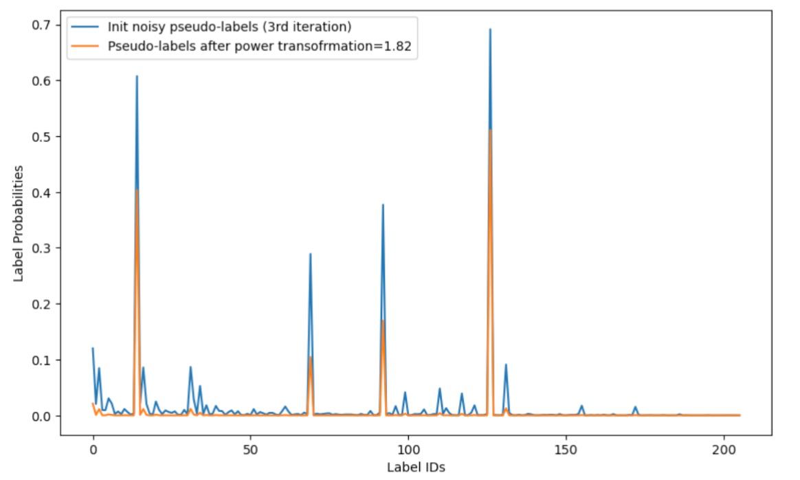\n\nKnowing how to train a multi-iterative noisy student, I ran 4 iterations, adjusting the pseudo-label power at each stage by validating results on the LB and consistently got the LB boost.\nThat self-training magic stopped working on the 5th pseudo-labeling iteration. I could not achieve any further improvement, so I stopped with the attempts to make new iterations work.\n|Iteration | Power value | Public LB |\n| --- | --- | --- |\n| 1 | 1 | 0.909 |\n| 2 |1 / 0.65 | 0.918 |\n| 3 | 1 / 0.55 | 0.927 |\n| **4** | **1 / 0.6** | **0.93** |\n\n#### Training Details\n- Besides extending the training ensemble with eca_nfnet_l0, efficientnet4, and applying power to labels, all training details remained unchanged since the 1st iteration.\n\n### Separate model for Amphibia and Insecta\nKnowing that species groups like Amphibia and Insecta are very underrepresented, and that Xeno-Canto provides data for multiple species from those groups that are not present in the train, I decided to try training a separate model that would see samples only from those groups, with a much higher diversity of species. The motivation was that the model would learn more representative features relevant to those groups, which would be a great supplement to the models that are trained only on a restricted number of samples/species from the training data.\n\n#### Data details\n- Species groups: amphibia, insecta\n- Total number of species: 700\n- Total number of samples: 17844\n- Data sources: train, xeno-canto samples that are shorter than 1 minute\n- Minimum number of samples per species: 1 (raising that value to 5 dropped scores a lot)\n\n#### Training Details\n- Epochs: 40\n- BS: 128 (with lower value scores dropped)\n- Model: efficient net 0 ns (deeper models and ensembles did not work much)\n- Other parameters are the same as for other models from my solution\n\n#### Inference Details\n- Run inference for all species\n- Insert predictions for target species into a zero matrix, only their columns are non-zero, for ensembling with other models\n\nAfter finding the optimal working parameters, I achieved a 0.002–0.003 LB boost.\n\n### Final Ensemble\nI found that ensembling models from different training stages was beneficial not only for slightly improving the LB score, but also for giving me a little confidence that my solution is not overfitted by doing more and more self-training iterations. \n\nThe final ensemble consisted of the following **7 models** trained on the specific data and different self-training iterations:\n- 1 efficientnetb4 from 3rd self-training iteration\n- 1 efficientnetb3 from 3rd self-training iteration\n- 2 regnety016 from 4th self-training iteration\n- 1 ecanfnetl0 from 3rd self-training iteration(with additional Xeno-Canto data for target species)\n- 1 regnety008 from 1 stage(supervised training)\n- 1 efficientnetb0 (supervised training on the extended Amphibia/Insecta species) \n\nIn my best solution, I tweaked the ensembling weights a bit, giving to efficientnetb3 and ecanfnetl0 slightly higher weights since they performed better as single models. However, the best private submission, with a score of 0.935, was achieved when I assigned equal weights to all models.\n\n**I believe that the ensembling of multi-stage models, diverse backbone architectures, and the dedicated model to certain species groups were crucial parts of my solution to withstanding the shake-up.**\nAs a result, my best public LB score dropped only slightly on the private LB **from 0.933 to 0.930**.\n\n### Inference optimization\n- OpenVINO inference engine without quantization\n- Multiprocess loading of the test soundscapes \n- Spectrograms were generated once and then reused across all models\n\n### Closing words\nI apologize that my write-up turned out to be a bit long. I did not want to skip anything important. \nMy Google Sheet accumulated during the competition over 320+ rows of ideas to check (95% of which were eventually marked red). So I decided not to include the `What did not work` block, otherwise it would significantly increase the length of the already long write-up.\nPlease feel free to ask me any questions about my solution in the comments. I will do my best to answer them.\n\nI also want to thank all the participants of the previous BirdCLEF iterations who shared their ideas.\nWithout your brilliant ideas, I would not have been able to achieve that result.\n\nSpecial thanks to the organizers, hosts, and everyone involved in conducting BirdCLEF. It is very appreciated that you put so much effort into conducting BirdCLEF each year, that you constantly stay in touch, and make each new iteration special(which is reflected in this year's number of participants).\n\n### References\n[1] [Self-training with Noisy Student improves ImageNet classification](https://arxiv.org/abs/1911.04252)\n[2] [Design Choices for Enhancing Noisy Student Self-Training](https://openaccess.thecvf.com/content/WACV2024/papers/Radhakrishnan_Design_Choices_for_Enhancing_Noisy_Student_Self-Training_WACV_2024_paper.pdf)\n[3] [Deep Networks with Stochastic Depth](https://arxiv.org/abs/1603.09382)\n\n### Resources \nInference notebook: https://www.kaggle.com/code/nikitababich/birdclef2025-1st-place-inference\nDatasets: [Extra Xeno-Canto data used in the solution ](https://www.kaggle.com/datasets/nikitababich/birdclef2025-1st-place-extra-data)", "votes": 263 }, { "id": 3223603, "postDate": "2025-06-13T14:44:06.360Z", "content": "Hoping good luck with you and your country. I looked your solution on EEDI, hoping world to be peace.
", "rawMarkdown": "Hoping good luck with you and your country. I looked your solution on EEDI, hoping world to be peace.", "votes": 7 }, { "id": 3219582, "postDate": "2025-06-08T02:24:34.700Z", "content": "Congratulations for the amazing feat winning this competition!!
\nNot to forget, winning in such adverse situation makes the win even more grand.
\nMy constant prayers for yours' and your families' safety.
@nikitababich Thank you again for your fantastic BirdCLEF 2025 solution write-up! I'm trying to replicate parts of it and have a few very specific questions about your Stage 1 (Supervised Learning):
\nQuestion 1: Gradient Clipping (max_grad_norm)
max_grad_norm value)?max_grad_norm?Question 2: Loss Function Structure (Stage 1)
\nYou mentioned using CrossEntropy (CE) loss for Stage 1. My current understanding for implementing a combined loss for an SED model is as follows. Could you please let me know if this aligns with your approach for Stage 1, or how your CE loss structure differed?
\n ():\n losses = {}\n losses[] = .criterions[](\n torch.logit(outputs[]),labels\n )\n losses[] = .criterions[](\n outputs[].()[], labels\n )\n losses[] = *losses[] + losses[] * \n losses\nQuestion 3: Stage 1 MixUp Padding Code
\nYour clarification on these specific points for Stage 1 would be extremely helpful.
\nThank you for your time and willingness to share!
Hi @lhr124578
\n1) Regarding Gradient Clipping - I was checking gradient norms during training and did not see any dangerous fluctuations, so I stepped back from using it.
\n2) Your loss implementation is the one that I used.
\n3) Here is my padding function:
():\n wave_init_len = wave.shape[]\n\n wave_init_len >= expected_len:\n wave[:expected_len]\n\n pad_len = expected_len - wave_init_len\n\n pad_type == :\n padded_wave = np.zeros(expected_len, dtype=wave.dtype)\n insert_wave_start = np.random.randint(, pad_len + )\n padded_wave[insert_wave_start: insert_wave_start + wave_init_len] = wave\n padded_wave\n\n pad_type == :\n np.pad(wave, ((pad_len, )))\n\n pad_type == :\n reps = (np.ceil(expected_len / wave_init_len))\n repeated = np.tile(wave, reps)\n repeated[:expected_len]\n\n :\n ValueError()\n@nikitababich
\nThank you so much for taking the time to reply and for your incredibly helpful clarifications on my previous questions regarding gradient clipping, the loss function structure, and the MixUp padding in your Stage 1 setup! Your detailed explanations are invaluable.
I have a couple of quick follow-up questions based on re-reading your solution and general data processing considerations:
\nHuman Voice Removal: Regarding the audio data (both the focal training data and the soundscapes used for pseudo-labeling, which you mentioned were normalized by absmax before MixUp), I noticed there wasn't a specific mention of further pre-processing steps like human voice removal .Could you perhaps share your thoughts or experience on this?
MixUp Target Handling: When applying MixUp to the absmax normalized audio waves (as mentioned for Stage 1), how were the corresponding target labels handled?
mixed_target = lambda * target1 + (1 - lambda) * target2@lhr124578
\n1) I did not succeed with the preprocessing of CSA, and any attempt to remove human voice deteriorated the results. I hypothesize that most of the underrepresented species, whose samples are extremely noisy, are not present in the hidden data. So, when we filter out noise (human voice) from the samples of those species (which make up most of the duration of those samples), we are left with very short single calls that lack much of the surrounding context. These short calls are indistinguishable from parts of calls of other, more represented CSA species, making the preprocessing detrimental to training on those other species.
2) The maximum between targets was taken in all MixUps, whether it was train + train or train + pseudo.
", "rawMarkdown": "@lhr124578 \n1) I did not succeed with the preprocessing of CSA, and any attempt to remove human voice deteriorated the results. I hypothesize that most of the underrepresented species, whose samples are extremely noisy, are not present in the hidden data. So, when we filter out noise (human voice) from the samples of those species (which make up most of the duration of those samples), we are left with very short single calls that lack much of the surrounding context. These short calls are indistinguishable from parts of calls of other, more represented CSA species, making the preprocessing detrimental to training on those other species.\n\n2) The maximum between targets was taken in all MixUps, whether it was train + train or train + pseudo.", "votes": 1 } ] } ] }, { "id": 3224604, "postDate": "2025-06-15T06:40:49.240Z", "content": "Huge congrats on your first-place win! What you pulled off is even more amazing given the incredibly tough situation you were in.
\nThanks for sharing how you did it. Your insights are super valuable to the community and will definitely help everyone learn and grow.
\nI was really moved by what you shared about your reality during the competition. Finishing your final submissions from a shelter during an attack? That shows incredible grit and determination. It's a powerful reminder of how resilient people can be, pushing for excellence even when things are incredibly hard.
\nYour shout-out to the Armed Forces of Ukraine, Security Service, Defence Intelligence, and State Emergency Service really highlights the crucial support that made your participation possible. Their work keeping people safe and secure didn't just protect lives; it also let you contribute to science and tech progress despite the ongoing conflict.
\nYour story is a powerful testament to simply not giving up. Thanks for not only sharing your technical know-how but also for giving us this important look at your journey to victory.
", "rawMarkdown": "**Huge congrats on your first-place win!** What you pulled off is even more amazing given the incredibly tough situation you were in.\n\nThanks for sharing how you did it. Your insights are super valuable to the community and will definitely help everyone learn and grow.\n\nI was really moved by what you shared about your reality during the competition. Finishing your final submissions from a shelter during an attack? That shows incredible grit and determination. It's a powerful reminder of how resilient people can be, pushing for excellence even when things are incredibly hard.\n\nYour shout-out to the Armed Forces of Ukraine, Security Service, Defence Intelligence, and State Emergency Service really highlights the crucial support that made your participation possible. Their work keeping people safe and secure didn't just protect lives; it also let you contribute to science and tech progress despite the ongoing conflict.\n\nYour story is a powerful testament to simply not giving up. Thanks for not only sharing your technical know-how but also for giving us this important look at your journey to victory.", "votes": 1 }, { "id": 3220950, "postDate": "2025-06-10T07:32:27.130Z", "content": "Great… what a remarkable work!
", "rawMarkdown": "Great... what a remarkable work!", "votes": 1 }, { "id": 3220627, "postDate": "2025-06-09T16:09:41.823Z", "content": "Amazing Bro!
", "rawMarkdown": "Amazing Bro!", "votes": 1 }, { "id": 3220371, "postDate": "2025-06-09T08:00:06.243Z", "content": "Congrats! It's great to see a winning solution, as someone who had recently started with Kaggle. It provides more motivation to grow, and learn from this community.
", "rawMarkdown": "Congrats! It's great to see a winning solution, as someone who had recently started with Kaggle. It provides more motivation to grow, and learn from this community. ", "votes": 1 }, { "id": 3220359, "postDate": "2025-06-09T07:44:35.593Z", "content": "Congrats!!That was really helpful
", "rawMarkdown": "Congrats!!That was really helpful", "votes": 1 }, { "id": 3220237, "postDate": "2025-06-09T03:50:30.750Z", "content": "Awesome! what a remarkable work!
", "rawMarkdown": "Awesome! what a remarkable work!", "votes": 1 }, { "id": 3219978, "postDate": "2025-06-08T15:38:41.297Z", "content": "Congratulations on an incredible 1st place solution, Nikita! This is truly impressive work and a fantastic write-up. Thank you for sharing such a detailed approach.
", "rawMarkdown": "Congratulations on an incredible 1st place solution, Nikita! This is truly impressive work and a fantastic write-up. Thank you for sharing such a detailed approach.", "votes": 1 }, { "id": 3219955, "postDate": "2025-06-08T15:11:43.397Z", "content": "Well done and thanks for sharing those insights! The iterative steps are very interesting.
", "rawMarkdown": "Well done and thanks for sharing those insights! The iterative steps are very interesting. ", "votes": 1 }, { "id": 3219665, "postDate": "2025-06-08T06:38:14.537Z", "content": "amazing! congratulations!
", "rawMarkdown": "amazing! congratulations!", "votes": 1 }, { "id": 3221528, "postDate": "2025-06-11T06:24:14.727Z", "content": "Thanks @nikitababich, a full engineering work!
", "rawMarkdown": "Thanks @nikitababich, a full engineering work!", "votes": 2 }, { "id": 3220660, "postDate": "2025-06-09T17:15:51.703Z", "content": "This thing is really helpful and thanks for sharing this.
", "rawMarkdown": "This thing is really helpful and thanks for sharing this.", "votes": 2 }, { "id": 3220215, "postDate": "2025-06-09T02:55:58.403Z", "content": "Congratulations on this well deserved win, the quality of work on display is remarkable. Nailing a win with this wide a margin especially while under extreme duress took a level of courage and fortitude that is rarely seen.
", "rawMarkdown": "Congratulations on this well deserved win, the quality of work on display is remarkable. Nailing a win with this wide a margin especially while under extreme duress took a level of courage and fortitude that is rarely seen.", "votes": 2 }, { "id": 3219947, "postDate": "2025-06-08T15:00:44.420Z", "content": "@nikitababich Congrats and you lead the Leaderboard in top almost 95% of the 3 months. New learnings from your solution - will try with late submissions.
\n\n\nIs it possible to share your experiments, which help as learning lesson to approach this competition of your My Google Sheet accumulated during the competition over 320+ rows of ideas to check (95% of which were eventually marked red).
\n
\n", "rawMarkdown": "@nikitababich **Congrats** and you **lead the Leaderboard in top almost 95% of the 3 months**. New learnings from your solution - will try with late submissions.\n\n> Is it possible to share your experiments, which help as learning lesson to approach this competition of your **My Google Sheet accumulated during the competition over 320+ rows of ideas to check (95% of which were eventually marked red).**\n\n---\n\n> Waiting for you Github, **Congrats once again with stable CV**.", "votes": 2, "replies": [ { "id": 3219976, "postDate": "2025-06-08T15:31:32.723Z", "content": "Waiting for you Github, Congrats once again with stable CV.
\n
Thank you @seshurajup
\nThat table is very messy, I do not think it can be understood as it is now:) But if you think that the chronology and progression of those ideas might be useful, I'll consider polishing and sharing that sheet.
Hi @nikitababich, any plans for release the github with your experiments?
", "rawMarkdown": "Hi @nikitababich, any plans for release the github with your experiments?" } ] } ] }, { "id": 3219835, "postDate": "2025-06-08T11:18:42.527Z", "content": "Congratulations and thank you for sharing Nikita, did you experiment with fmin and fmax at all?
", "rawMarkdown": "Congratulations and thank you for sharing Nikita, did you experiment with fmin and fmax at all?", "votes": 2, "replies": [ { "id": 3219964, "postDate": "2025-06-08T15:20:13.310Z", "content": "Thank you @lyndonreidd
\nIt is a good question.
\nInitially, I began with more \"usual\" mel parameters like MelSpectrogram(sample_rate: 32000, mel_bins: 128, fmin: 40, fmax: 15000, n_fft: 2048, hop_size: 512, top_db=80.0) and then step-by-step I tuned them based on the responses from the Public LB.
\nTalking specifically about fmin, fmax - adjusting them from (40, 15000) to (0, 16000) showed a very minor impact on the LB, so I did not play much with them after that.
\nI experienced a much more significant impact on the score by adjusting the following parameters: mel_bins, n_fft, hop_size ( you can check my explanation on why these adjustments were important in Thoughts on mel parameters tuning of my write-up).
Awesome! what a remarkable work. Be safe 💙
", "rawMarkdown": "Awesome! what a remarkable work. Be safe 💙", "votes": 2 }, { "id": 3219958, "postDate": "2025-06-08T15:17:20.247Z", "content": "Congratulations👏 for the amazing feat winning this competition!✨
", "rawMarkdown": "Congratulations👏 for the amazing feat winning this competition!✨" }, { "id": 3231932, "postDate": "2025-06-25T06:33:56.270Z", "content": "Thanks so much for sharing. My first time digging into competitive architectures in one of these competitions and I learned a ton!
", "rawMarkdown": "Thanks so much for sharing. My first time digging into competitive architectures in one of these competitions and I learned a ton! " }, { "id": 3231427, "postDate": "2025-06-24T10:21:35.107Z", "content": "Congratulations and thanks for sharing your work
", "rawMarkdown": "Congratulations and thanks for sharing your work" }, { "id": 3224732, "postDate": "2025-06-15T11:27:21.173Z", "content": "Amazing Work!!
", "rawMarkdown": "Amazing Work!!" }, { "id": 3224631, "postDate": "2025-06-15T08:00:57.437Z", "content": "Amazing Work!!
", "rawMarkdown": "Amazing Work!!" }, { "id": 3222426, "postDate": "2025-06-12T07:35:45.300Z", "content": "Amazing Work!!
", "rawMarkdown": "Amazing Work!!" }, { "id": 3222216, "postDate": "2025-06-12T02:54:37.747Z", "rawMarkdown": "", "isDeleted": true }, { "id": 3219662, "postDate": "2025-06-08T06:28:22.423Z", "rawMarkdown": "", "isDeleted": true }, { "id": 3221006, "postDate": "2025-06-10T09:07:57.350Z", "content": "Nice Work !!
", "rawMarkdown": "Nice Work !!", "votes": 2 }, { "id": 3221100, "postDate": "2025-06-10T11:53:28.803Z", "content": "Thanks for sharing!
", "rawMarkdown": "Thanks for sharing!", "votes": 1 }, { "id": 3231169, "postDate": "2025-06-24T03:01:07.507Z", "content": "Great Job🤗
", "rawMarkdown": "Great Job🤗" }, { "id": 3224658, "postDate": "2025-06-15T09:14:42.107Z", "content": "Respectful! Thank you for your sharing!
", "rawMarkdown": "Respectful! Thank you for your sharing!" }, { "id": 3221961, "postDate": "2025-06-11T16:21:59.257Z", "content": "Thank you , it is a great work!!!
", "rawMarkdown": "Thank you , it is a great work!!!\n" }, { "id": 3221930, "postDate": "2025-06-11T15:54:51.510Z", "content": "Thanks for sharing..
", "rawMarkdown": "Thanks for sharing.. " } ], "comments": [ { "id": 3223603, "author_name": "Kurise", "author_url": "", "post_date": "2025-06-13T14:44:06.360000", "content": "Hoping good luck with you and your country. I looked your solution on EEDI, hoping world to be peace.
", "votes": 7, "replies": [] }, { "id": 3219582, "author_name": "Aayush Kumar Singha", "author_url": "", "post_date": "2025-06-08T02:24:34.700000", "content": "Congratulations for the amazing feat winning this competition!!
\nNot to forget, winning in such adverse situation makes the win even more grand.
\nMy constant prayers for yours' and your families' safety.
@nikitababich Thank you again for your fantastic BirdCLEF 2025 solution write-up! I'm trying to replicate parts of it and have a few very specific questions about your Stage 1 (Supervised Learning):
\nQuestion 1: Gradient Clipping (max_grad_norm)
max_grad_norm value)?max_grad_norm?Question 2: Loss Function Structure (Stage 1)
\nYou mentioned using CrossEntropy (CE) loss for Stage 1. My current understanding for implementing a combined loss for an SED model is as follows. Could you please let me know if this aligns with your approach for Stage 1, or how your CE loss structure differed?
\n ():\n losses = {}\n losses[] = .criterions[](\n torch.logit(outputs[]),labels\n )\n losses[] = .criterions[](\n outputs[].()[], labels\n )\n losses[] = *losses[] + losses[] * \n losses\nQuestion 3: Stage 1 MixUp Padding Code
\nYour clarification on these specific points for Stage 1 would be extremely helpful.
\nThank you for your time and willingness to share!
Hi @lhr124578
\n1) Regarding Gradient Clipping - I was checking gradient norms during training and did not see any dangerous fluctuations, so I stepped back from using it.
\n2) Your loss implementation is the one that I used.
\n3) Here is my padding function:
():\n wave_init_len = wave.shape[]\n\n wave_init_len >= expected_len:\n wave[:expected_len]\n\n pad_len = expected_len - wave_init_len\n\n pad_type == :\n padded_wave = np.zeros(expected_len, dtype=wave.dtype)\n insert_wave_start = np.random.randint(, pad_len + )\n padded_wave[insert_wave_start: insert_wave_start + wave_init_len] = wave\n padded_wave\n\n pad_type == :\n np.pad(wave, ((pad_len, )))\n\n pad_type == :\n reps = (np.ceil(expected_len / wave_init_len))\n repeated = np.tile(wave, reps)\n repeated[:expected_len]\n\n :\n ValueError()\n@nikitababich
\nThank you so much for taking the time to reply and for your incredibly helpful clarifications on my previous questions regarding gradient clipping, the loss function structure, and the MixUp padding in your Stage 1 setup! Your detailed explanations are invaluable.
I have a couple of quick follow-up questions based on re-reading your solution and general data processing considerations:
\nHuman Voice Removal: Regarding the audio data (both the focal training data and the soundscapes used for pseudo-labeling, which you mentioned were normalized by absmax before MixUp), I noticed there wasn't a specific mention of further pre-processing steps like human voice removal .Could you perhaps share your thoughts or experience on this?
MixUp Target Handling: When applying MixUp to the absmax normalized audio waves (as mentioned for Stage 1), how were the corresponding target labels handled?
mixed_target = lambda * target1 + (1 - lambda) * target2@lhr124578
\n1) I did not succeed with the preprocessing of CSA, and any attempt to remove human voice deteriorated the results. I hypothesize that most of the underrepresented species, whose samples are extremely noisy, are not present in the hidden data. So, when we filter out noise (human voice) from the samples of those species (which make up most of the duration of those samples), we are left with very short single calls that lack much of the surrounding context. These short calls are indistinguishable from parts of calls of other, more represented CSA species, making the preprocessing detrimental to training on those other species.
2) The maximum between targets was taken in all MixUps, whether it was train + train or train + pseudo.
", "votes": 1, "replies": [] } ] } ] }, { "id": 3224604, "author_name": "Pablo Yelloworld", "author_url": "", "post_date": "2025-06-15T06:40:49.240000", "content": "Huge congrats on your first-place win! What you pulled off is even more amazing given the incredibly tough situation you were in.
\nThanks for sharing how you did it. Your insights are super valuable to the community and will definitely help everyone learn and grow.
\nI was really moved by what you shared about your reality during the competition. Finishing your final submissions from a shelter during an attack? That shows incredible grit and determination. It's a powerful reminder of how resilient people can be, pushing for excellence even when things are incredibly hard.
\nYour shout-out to the Armed Forces of Ukraine, Security Service, Defence Intelligence, and State Emergency Service really highlights the crucial support that made your participation possible. Their work keeping people safe and secure didn't just protect lives; it also let you contribute to science and tech progress despite the ongoing conflict.
\nYour story is a powerful testament to simply not giving up. Thanks for not only sharing your technical know-how but also for giving us this important look at your journey to victory.
", "votes": 1, "replies": [] }, { "id": 3220950, "author_name": "Sarah Arshad", "author_url": "", "post_date": "2025-06-10T07:32:27.130000", "content": "Great… what a remarkable work!
", "votes": 1, "replies": [] }, { "id": 3220627, "author_name": "Devendra Jadhav", "author_url": "", "post_date": "2025-06-09T16:09:41.823000", "content": "Amazing Bro!
", "votes": 1, "replies": [] }, { "id": 3220371, "author_name": "aaaditya56", "author_url": "", "post_date": "2025-06-09T08:00:06.243000", "content": "Congrats! It's great to see a winning solution, as someone who had recently started with Kaggle. It provides more motivation to grow, and learn from this community.
", "votes": 1, "replies": [] }, { "id": 3220359, "author_name": "Ten-Mergen Gandavaa", "author_url": "", "post_date": "2025-06-09T07:44:35.593000", "content": "Congrats!!That was really helpful
", "votes": 1, "replies": [] }, { "id": 3220237, "author_name": "zhuzhu521", "author_url": "", "post_date": "2025-06-09T03:50:30.750000", "content": "Awesome! what a remarkable work!
", "votes": 1, "replies": [] }, { "id": 3219978, "author_name": "Aniket Potabatti", "author_url": "", "post_date": "2025-06-08T15:38:41.297000", "content": "Congratulations on an incredible 1st place solution, Nikita! This is truly impressive work and a fantastic write-up. Thank you for sharing such a detailed approach.
", "votes": 1, "replies": [] }, { "id": 3219955, "author_name": "Yassine Alouini", "author_url": "", "post_date": "2025-06-08T15:11:43.397000", "content": "Well done and thanks for sharing those insights! The iterative steps are very interesting.
", "votes": 1, "replies": [] }, { "id": 3219665, "author_name": "Matheus Parracho", "author_url": "", "post_date": "2025-06-08T06:38:14.537000", "content": "amazing! congratulations!
", "votes": 1, "replies": [] }, { "id": 3221528, "author_name": "Victor Caquilpan", "author_url": "", "post_date": "2025-06-11T06:24:14.727000", "content": "Thanks @nikitababich, a full engineering work!
", "votes": 2, "replies": [] }, { "id": 3220660, "author_name": "Harsh Gupta", "author_url": "", "post_date": "2025-06-09T17:15:51.703000", "content": "This thing is really helpful and thanks for sharing this.
", "votes": 2, "replies": [] }, { "id": 3220215, "author_name": "Bilal A. Chaudhry", "author_url": "", "post_date": "2025-06-09T02:55:58.403000", "content": "Congratulations on this well deserved win, the quality of work on display is remarkable. Nailing a win with this wide a margin especially while under extreme duress took a level of courage and fortitude that is rarely seen.
", "votes": 2, "replies": [] }, { "id": 3219947, "author_name": "SeshuRaju 🧘♂️", "author_url": "", "post_date": "2025-06-08T15:00:44.420000", "content": "@nikitababich Congrats and you lead the Leaderboard in top almost 95% of the 3 months. New learnings from your solution - will try with late submissions.
\n\n\nIs it possible to share your experiments, which help as learning lesson to approach this competition of your My Google Sheet accumulated during the competition over 320+ rows of ideas to check (95% of which were eventually marked red).
\n
\n", "votes": 2, "replies": [ { "id": 3219976, "author_name": "Nikita Babych", "author_url": "", "post_date": "2025-06-08T15:31:32.723000", "content": "Waiting for you Github, Congrats once again with stable CV.
\n
Thank you @seshurajup
\nThat table is very messy, I do not think it can be understood as it is now:) But if you think that the chronology and progression of those ideas might be useful, I'll consider polishing and sharing that sheet.
Hi @nikitababich, any plans for release the github with your experiments?
", "votes": 0, "replies": [] } ] } ] }, { "id": 3219835, "author_name": "Lyndon Reid", "author_url": "", "post_date": "2025-06-08T11:18:42.527000", "content": "Congratulations and thank you for sharing Nikita, did you experiment with fmin and fmax at all?
", "votes": 2, "replies": [ { "id": 3219964, "author_name": "Nikita Babych", "author_url": "", "post_date": "2025-06-08T15:20:13.310000", "content": "Thank you @lyndonreidd
\nIt is a good question.
\nInitially, I began with more \"usual\" mel parameters like MelSpectrogram(sample_rate: 32000, mel_bins: 128, fmin: 40, fmax: 15000, n_fft: 2048, hop_size: 512, top_db=80.0) and then step-by-step I tuned them based on the responses from the Public LB.
\nTalking specifically about fmin, fmax - adjusting them from (40, 15000) to (0, 16000) showed a very minor impact on the LB, so I did not play much with them after that.
\nI experienced a much more significant impact on the score by adjusting the following parameters: mel_bins, n_fft, hop_size ( you can check my explanation on why these adjustments were important in Thoughts on mel parameters tuning of my write-up).
Awesome! what a remarkable work. Be safe 💙
", "votes": 2, "replies": [] }, { "id": 3219958, "author_name": "Khushi Yadav", "author_url": "", "post_date": "2025-06-08T15:17:20.247000", "content": "Congratulations👏 for the amazing feat winning this competition!✨
", "votes": 0, "replies": [] }, { "id": 3231932, "author_name": "Tom Madden", "author_url": "", "post_date": "2025-06-25T06:33:56.270000", "content": "Thanks so much for sharing. My first time digging into competitive architectures in one of these competitions and I learned a ton!
", "votes": 0, "replies": [] }, { "id": 3231427, "author_name": "Shashi1024", "author_url": "", "post_date": "2025-06-24T10:21:35.107000", "content": "Congratulations and thanks for sharing your work
", "votes": 0, "replies": [] }, { "id": 3224732, "author_name": "Dasun Weerakoon", "author_url": "", "post_date": "2025-06-15T11:27:21.173000", "content": "Amazing Work!!
", "votes": 0, "replies": [] }, { "id": 3224631, "author_name": "Hamza Bashir", "author_url": "", "post_date": "2025-06-15T08:00:57.437000", "content": "Amazing Work!!
", "votes": 0, "replies": [] }, { "id": 3222426, "author_name": "", "author_url": "", "post_date": "2025-06-12T07:35:45.300000", "content": "Amazing Work!!
", "votes": 0, "replies": [] }, { "id": 3222216, "author_name": "", "author_url": "", "post_date": "2025-06-12T02:54:37.747000", "content": "", "votes": 0, "replies": [] }, { "id": 3219662, "author_name": "", "author_url": "", "post_date": "2025-06-08T06:28:22.423000", "content": "", "votes": 0, "replies": [] }, { "id": 3221006, "author_name": "Mansik Rehman", "author_url": "", "post_date": "2025-06-10T09:07:57.350000", "content": "Nice Work !!
", "votes": 2, "replies": [] }, { "id": 3221100, "author_name": "Khushi Yadav", "author_url": "", "post_date": "2025-06-10T11:53:28.803000", "content": "Thanks for sharing!
", "votes": 1, "replies": [] }, { "id": 3231169, "author_name": "HaogeBob", "author_url": "", "post_date": "2025-06-24T03:01:07.507000", "content": "Great Job🤗
", "votes": 0, "replies": [] }, { "id": 3224658, "author_name": "", "author_url": "", "post_date": "2025-06-15T09:14:42.107000", "content": "", "votes": 0, "replies": [] }, { "id": 3221961, "author_name": "", "author_url": "", "post_date": "2025-06-11T16:21:59.257000", "content": "", "votes": 0, "replies": [] }, { "id": 3221930, "author_name": "", "author_url": "", "post_date": "2025-06-11T15:54:51.510000", "content": "", "votes": 0, "replies": [] } ], "raw_markdown_by_id": { "3219545": ">I know that Kagglers are aware of what’s happening in Ukraine, and you’re here to take a look at my solution, but let me share a small glimpse from the competition’s deadline day that reflects our current reality: I had to make my final submissions from a shelter while we had a stable connection, as Ukraine was under another devastating attack with many civilian casualties, some of them from my neighborhood. \n*I would like to thank the Armed Forces of Ukraine, Security Service of Ukraine, Defence Intelligence of Ukraine, and the State Emergency Service of Ukraine for providing safety and security to participate in this great competition, complete this work, and help science, technology, and business not to stop but to move forward.*\n\n## TLDR\n- SED models on 20-second input chunks.\n- A Multi-Iterative Noisy Student is used as a self-training approach via MixUp between focal training data and pseudo-labeled soundscapes.\n- Power transform applied to pseudo-labels to reduce noise.\n- Pseudo-label sampler assigns weights equal to the sum of the maximum of labels within each soundscape.\n- A separate model for Amphibia and Insecta label groups using extended species data from Xeno-Canto.\n- A final ensemble with models from different training iterations.\n- Inference is performed by averaging overlapping framewise predictions from neighboring chunks, followed by smoothing and delta shift inference.\n\n## Solution Overview\n.png?generation=1749292477050741&alt=media)\n\n### Data\n#### Additional Xeno-Canto Data\n- Target species\n - Num samples: 5489\n - Samples per species groups: Aves(birds)=5480, Amphibia=6, Mammalia=3\n - Max samples per species: 500\n - Comment: It usually worsened results, so only one model saw that data.\n- Extra species \n - Num samples: 17197\n - Samples per species groups: Insecta=16218(544 extra species), Amphibia=979(113 extra species)\n - Max samples per species: 200\n - Additional filters: duration less than 60 sec\n - Comment: This data was used to train a separate dedicated model for the Insecta and Amphibia groups.\n\n#### Interesting note about Insecta\nThe Insecta group included labels at the family level, such as Cicadidae, Gryllidae, and Tettigoniidae, while the rest of the Insecta labels were species from the Tettigoniidae family. But the following experiments showed that the family-level labels were probably related to the specific species or at least to a narrow set of species that inhabit the Middle Magdalena Valley:\n- Including the Tettigoniidae label in secondary labels of species from the Tettigoniidae family worsened results. \n- Including extra Xeno-Canto data for Gryllidae and Tettigoniidae (i.e., family-level labels) in training on target species also worsened results.\n- Using additional Gryllidae and Tettigoniidae samples from Xeno-Canto, assigning them unique new labels based on the species of each sample instead of assigning the family-level labels, and training a dedicated model improved results. It means that Tettigoniidae and Gryllidae target labels are related to the specific species that can be separated from other species within these families that are present as other Insecta target labels or extra species from these families that were downloaded.\n\n####Data preparation\n- 5 folds\n- Each fold includes at least 1 sample for each label\n- 20-second audio chunks normalized by absmax\n- All secondary labels = 1\n\nFrom the start, I came to the thought that the presence of Amphibia and Insecta groups would make models favor longer input durations over shorter ones, since the long duration and repetitiveness of their calls are distinctive features for species from these groups.\nTo find the most optimal duration, I conducted multiple experiments with different durations and figured that 20-second chunks work best for me, and any longer duration did not improve results but took more time to infer, so I continued with that chunk duration. \nHere are the Public scores that I obtained by experimenting with different durations while training(supervised with train data only) an ensemble of 5 SED efficientnetb0 models and adjusting proportionally spectrogram hop length(more detailed information on the models and inference is provided in the next sections):\n| Chunk duration | Public LB |\n| --- | --- |\n|5 sec | 0.842 |\n|10 sec | 0.864 |\n|15 sec | 0.87 |\n|**20 sec** | **0.872** |\n|30 sec | 0.872 |\n\n### Models\n#### Architectures\nAcross different training stages, I used various CNNs, gradually incorporating more complex models at each stage. All models included the SED head (adaptation from [the 4th place 2021](https://www.kaggle.com/competitions/birdclef-2021/discussion/243293) ), which consistently provided a significant boost over other head variations.\n- SED \n- Gem frequency pooling \n- Repeated 3 Mel Spectrograms as input\n- 1 stage backbones: \n - tf_efficientnet_b0.ns_jft_in1k \n - regnety_008.pycls_in1k\n- 1 pseudo-labeling iteration backbones: \n - tf_efficientnet_b0.ns_jft_in1k \n - regnety_008.pycls_in1k\n - tf_efficientnet_b3.ns_jft_in1k \n - regnety_016.tv2_in1k\n- 2-4 pseudo-labeling iteration backbones: \n - tf_efficientnet_b3.ns_jft_in1k \n - tf_efficientnet_b4.ns_jft_in1k \n - regnety_016.tv2_in1k \n - eca_nfnet_l0.ra2_in1k\n- Amphibia/Insecta model backbone: \n - tf_efficientnet_b0.ns_jft_in1k \n\n#### Mel spectrogram parameters\n- 20 sec -> Image size = (3, 224, 512)\n- MelSpectrogram (sample_rate: 32000, mel_bins: 224, fmin: 0, fmax: 16000, n_fft: 4096, hop_size: 1252, top_db=80.0)\n- 0-1 normalization\n\n##### Thoughts on mel parameters tuning\n- Because long input chunks were used, I had to set a larger hop length value, otherwise, inference would take too long, and I wouldn’t have the capacity to prepare a good ensemble. \n- The important thing was setting a larger number of n_mels. I suspect this is because some species (especially from the Amphibia and Insecta groups) have calls within narrow frequency ranges, so showing more mel bands to models was important to distinguish species well.\n\n### Validation\n- I did not find a good CV/ LB correlation, so considering the Host's words that public/private distributions are very similar and the knowledge from last year's solutions, I validated ideas using only the public LB. \n- A single model’s LB score varied a lot for different seeds, so usually I trained the same setup on different folds(2-5, depending on the remaining time that I had) and ensembled them to obtain a more reliable response from the LB.\n\nAs it turned out, the Hosts were absolutely honest with us(did not have any doubt), and most Public results correlated pretty well with the private LB.\n\n### 1 Stage (Supervised Learning)\n#### Training Details \n- Epochs: 15\n- Loss: CrossEntropy\n- LR: 5e-4 - 1e-6(same for all models)\n- Optimizer: AdamW with 1e-4 weight decay\n- Scheduler: CosineAnnealingWarmRestarts with restart after each 5 epochs. Applying warm restarts, I could train longer than with one cycle\n- BS: 64\n- Augmentations: \n - Mixup: p = 0.5, on normalized by absmax raw audio with an equal sampling weight for each species\n- Padding: To keep samples of different lengths overlapping after mixup, the left part of it was filled with 0, so on the right, there is always an overlap that ensures train samples are always actually mixed up\n- Models: efficientnet0, regnety8. An ensemble of small models on the 1st stage gave almost the same results as ensembling deeper ones\n\n#### Loss choice\nI noticed that the choice of loss got a lot of attention in the discussions. So I conducted some experiments and found that both CE and BCE/Focal losses could give me similar results when the learning rate and the number of epochs were well-tuned. However, CE gave me a bit better results, so I settled on it.\nI connect better results with CE (I might be wrong) with the following interconnected assumptions: \n- The magnitude of updates with CE for each label depends on how well the positive labels (probability > 0) are classified. This means that if a rare positive label A gets a low probability, then the negative overrepresented label B(that has a higher probability than other negative labels) is pushed to zero with a stronger update. \n- CE handles imbalanced labels better and avoids overfitting to overrepresented classes by punishing them when Softmax can not give a higher score for A because the overrepresented label B already got too high logits as a result of the previous numerous imbalanced updates when label B was positive.\n\nAlso, I didn’t normalize sample labels to sum to one, motivated by the idea that more difficult samples (those with more positive labels) should have a greater impact on the loss.\n\n### Inference\n.png?generation=1749300190075357&alt=media)\n\nI am showing my inference flow first to give more context before going to the next sections, where I explain how I used pseudo-labels, which were generated with that inference. I hope my diagram does not look too overloaded. \nThe core idea was to fully leverage all framewise predictions produced by the SED head by averaging the overlapping framewise predictions from neighboring audio chunks, rather than taking max only from the central 5 sec and throwing away precious predictions.\n- It can be seen as a 1D analogue of 2D sliding-window segmentation of large images, rather than treating each audio chunk as a completely separate sample. \n- It can be seen as a form of test-time augmentation (TTA) because each framewise prediction is averaged over multiple chunks that present the same time frame to the model with slightly different surrounding context.\n- Consistently boosted my LB score (by 0.002-0.003).\n- Helped to get more generalizable predictions. \n\n#### Other inference/postprocessing tricks \n- Padded the left and right sides of the signal to ensure that the first and last 5-second chunks are centered after splitting. Framewise predictions related to the padding were then removed.\n- Smoothing [0.1, 0.2, 0.4, 0.2, 0.1].\n- Delta shift TTA (from [the 2nd solution 2023](https://www.kaggle.com/competitions/birdclef-2023/discussion/412707)).\n\n### Self-training \nAfter hitting the ceiling with the supervised approach, it became clear that further improvements would come with the usage of the unlabeled soundscapes. \nI pseudo-labeled the unlabeled data using the best LB ensemble from the 1 stage with the described above inference flow, and began experimenting with the ways to incorporate pseudo-labeled data in the training. \nInitial attempts to concatenate the pseudo-labeled data into training batches separately didn’t succeed. \n\n#### MixUps (finally working) \nThen I tried mixing up the pseudo-labeled raw data with the training raw data, following the approach from [the 2nd place solution 2024](https://www.kaggle.com/competitions/birdclef-2024/discussion/512340). At first, it didn’t work because I had set the Beta distribution’s parameters to be too low(used to sample blending weights). But after switching to a constant blending weight of 0.5(Beta’s parameters = inf), the magic started to happen, and the LB score began to rise. I suspect that is related to the fact that blending weights far from 0.5 sometimes suppress the meaningful signals, especially when mixing relatively clear train data with much noisier train soundscapes.\n\n##### Stochastic Depth\nReading the paper on the Noisy Student approach [1], I found certain similarities with the self-training approach I was using. \nSo, I started experimenting with the techniques that showed a positive impact on self-training in the mentioned paper and found that adding Stochastic Depth [3] (i.e., dropout applied to the entire residual blocks) worked for me as well.\n- Applying `drop_path_rate = 0.15` (which turned out to be optimal for all the models I trained), I consistently saw a boost in the LB score, up to 0.005 for some models. \n- Applying Stochastic Depth during supervised training didn’t lead to any improvement, which supports the idea that the current self-training approach is a form of Noisy Student self-training.\n\n#### Why Noisy Student? (my understanding)\n>After reading [1], I finally understood why mixup works while simple concatenation doesn’t. Since it closely matched my approach, I considered it a form of Noisy Student self-training and named my solution accordingly.\nPutting simply - showing to the model the same input and asking for the same output does not teach the student anything new, so in the best case it converges to the same results, in the worst case it accumulates error and the LB score drops (what I experienced). But when we inject noise(augmentations like mixup, drop paths) and ask to provide the same output as for the clean input, it starts learning more robust features instead of accumulating error. \nI imagined the following scenario: we have a pseudo-labeled sample where A is the true label, and B is the negative one. The teacher model predicts A ≈ 1 and B ≈ 0, but not exactly zero. If we repeatedly train on this same input, the model may start learning irrelevant features associated with B, simply because its score isn’t exactly zero. It may also overfit to some noise because of thinking that it is related to A. At the same time, it doesn’t offer anything new beyond what the teacher model has already seen and learned, so it doesn’t lead to any improvement.\nHowever, if we augment that sample, the student model must work harder to understand why the teacher gave a high score to A(an unaugmented input for the teacher). As a result, through this noisy student training, we force the model to focus on the most consistent, generalizable features relevant to A rather than memorizing noise associated with A and B.\nAlso, Noisy Student methodology involves including labeled samples in training (as I did), whose signals help guide the model toward better optima, especially during the early epochs.\nAnd MixUps with pseudo-labeled data serve as a great augmentation for labeled samples, providing target domain backgrounds with soft-labels for possible species in that background.\n\n#### Pseudo-labels preparation\n- Pseudo-labels were generated using the best ensemble of models from the previous stage.\n- Pseudo-labels were generated before self-training and stored as max label probabilities for 5-second segments, or framewise predictions were stored as they are without pooling(4 frames per 5-second segment).\n- Framewise predictions provided more splits of soundscapes into chunks(9 splits for 20-second chunks when save for each 5 sec, and 45 splits when save framewise predictions), but more splits usually did not provide better results\n\n#### Pseudo-labeled data sampling\n- Soundscapes with a higher sum of maximum label probabilities were usually pseudo-labeled more accurately. This is because most soundscapes were overloaded with various species calls, and a low sum often indicated that the models struggled to recognize and distinguish those species. \n- WeightedRandomSampler was used with weights equal to the sum of maximum label probabilities within each soundscape. This ensured that samples with more accurate pseudo-labels were sampled more frequently. Idea to use a sampler for pseudo-labels, I found in that paper [2].\n - A random 20-second interval was selected from the training soundscape that was sampled by WeightedRandomSampler. \n - For that interval, the maximum probability for each label was taken across the 4 segments (or 16 frames), and then that soft labels were used in self-training. \n - WeightedRandomSampler stabilized training and boosted the LB score.\n - This approach was especially relevant after I reduced label noise (described in *Multi-Iterative pseudo-labeling* section) and ended up with many samples that had low label sums (less than 0.5 summing 206 labels), which was the same as using unlabeled data, so it was beneficial to give lower weights in sampling for such \"almost\" unlabeled samples.\n\n#### Training Details:\n- More epochs = 25-35.\n- Drop path rate = 0.15.\n- Random padding. Samples shorter than 20 sec were placed at random positions within 20 sec.\n- Other training parameters are the same as in supervised learning.\n\n#### Ratio of pseudo-labeled mixups\n- The ratio of labeled train samples that I mixed up with pseudo-labeled chunks in each batch(bs=64) was very important and significantly impacted the LB score. \n- To find the optimal ratio, I was gradually increasing it by 0.25, retraining an ensemble of 5 SED efficientnetb0 folds with the self-training setup described above, and checking the LB to find the best ratio.\n\n| Ratio of mixed samples| Public LB |\n| --- | --- |\n| 0 (labeled training data only) | 0.872 |\n| 0.25 | 0.883 |\n| 0.5 | 0.887 |\n| 0.75 | 0.89 |\n| **1.0** | **0.898** |\n\n- Turned out that mixing every training sample with a random pseudo-labeled sample showed the best score.\n\n### Multi-Iterative pseudo-labeling\nInspired by [the 2nd place solution 2024](https://www.kaggle.com/competitions/birdclef-2024/discussion/512340) and papers on self-training [1, 2], I tried to pseudo-label the unlabeled soundscapes again, using models that were already trained on the pseudo-labels from the previous iteration. However, this approach didn’t work out of the box, and I spent some time investigating why until I found the correct preprocessing of the pseudo-labels that allowed me to keep training models on the next pseudo-labeling iterations. \n\n#### Multi-Iterative labels preprocessing\nThe reason the models failed to converge in later iterations was that the pseudo-labels had become too noisy, obscuring any meaningful signal. \nHere is the method that worked best for me and allowed me to move forward:\n- The trick was to apply a power greater than 1 to the probabilities (similar to temperature scaling, but applied to probabilities instead of logits). This worked because applying temperature to logits increases probabilities above 0.5, which was deteriorating.\n- Applying the power to the probabilities, I was able to preserve the important signals while preventing the amplification of confident noise.\n\nIn the image below, you can see that the power transform is a real power in the fight against label noise. After the transformation, labels become much cleaner, and only initially confident labels survive, having still pronounced values to train models.\n\n\nKnowing how to train a multi-iterative noisy student, I ran 4 iterations, adjusting the pseudo-label power at each stage by validating results on the LB and consistently got the LB boost.\nThat self-training magic stopped working on the 5th pseudo-labeling iteration. I could not achieve any further improvement, so I stopped with the attempts to make new iterations work.\n|Iteration | Power value | Public LB |\n| --- | --- | --- |\n| 1 | 1 | 0.909 |\n| 2 |1 / 0.65 | 0.918 |\n| 3 | 1 / 0.55 | 0.927 |\n| **4** | **1 / 0.6** | **0.93** |\n\n#### Training Details\n- Besides extending the training ensemble with eca_nfnet_l0, efficientnet4, and applying power to labels, all training details remained unchanged since the 1st iteration.\n\n### Separate model for Amphibia and Insecta\nKnowing that species groups like Amphibia and Insecta are very underrepresented, and that Xeno-Canto provides data for multiple species from those groups that are not present in the train, I decided to try training a separate model that would see samples only from those groups, with a much higher diversity of species. The motivation was that the model would learn more representative features relevant to those groups, which would be a great supplement to the models that are trained only on a restricted number of samples/species from the training data.\n\n#### Data details\n- Species groups: amphibia, insecta\n- Total number of species: 700\n- Total number of samples: 17844\n- Data sources: train, xeno-canto samples that are shorter than 1 minute\n- Minimum number of samples per species: 1 (raising that value to 5 dropped scores a lot)\n\n#### Training Details\n- Epochs: 40\n- BS: 128 (with lower value scores dropped)\n- Model: efficient net 0 ns (deeper models and ensembles did not work much)\n- Other parameters are the same as for other models from my solution\n\n#### Inference Details\n- Run inference for all species\n- Insert predictions for target species into a zero matrix, only their columns are non-zero, for ensembling with other models\n\nAfter finding the optimal working parameters, I achieved a 0.002–0.003 LB boost.\n\n### Final Ensemble\nI found that ensembling models from different training stages was beneficial not only for slightly improving the LB score, but also for giving me a little confidence that my solution is not overfitted by doing more and more self-training iterations. \n\nThe final ensemble consisted of the following **7 models** trained on the specific data and different self-training iterations:\n- 1 efficientnetb4 from 3rd self-training iteration\n- 1 efficientnetb3 from 3rd self-training iteration\n- 2 regnety016 from 4th self-training iteration\n- 1 ecanfnetl0 from 3rd self-training iteration(with additional Xeno-Canto data for target species)\n- 1 regnety008 from 1 stage(supervised training)\n- 1 efficientnetb0 (supervised training on the extended Amphibia/Insecta species) \n\nIn my best solution, I tweaked the ensembling weights a bit, giving to efficientnetb3 and ecanfnetl0 slightly higher weights since they performed better as single models. However, the best private submission, with a score of 0.935, was achieved when I assigned equal weights to all models.\n\n**I believe that the ensembling of multi-stage models, diverse backbone architectures, and the dedicated model to certain species groups were crucial parts of my solution to withstanding the shake-up.**\nAs a result, my best public LB score dropped only slightly on the private LB **from 0.933 to 0.930**.\n\n### Inference optimization\n- OpenVINO inference engine without quantization\n- Multiprocess loading of the test soundscapes \n- Spectrograms were generated once and then reused across all models\n\n### Closing words\nI apologize that my write-up turned out to be a bit long. I did not want to skip anything important. \nMy Google Sheet accumulated during the competition over 320+ rows of ideas to check (95% of which were eventually marked red). So I decided not to include the `What did not work` block, otherwise it would significantly increase the length of the already long write-up.\nPlease feel free to ask me any questions about my solution in the comments. I will do my best to answer them.\n\nI also want to thank all the participants of the previous BirdCLEF iterations who shared their ideas.\nWithout your brilliant ideas, I would not have been able to achieve that result.\n\nSpecial thanks to the organizers, hosts, and everyone involved in conducting BirdCLEF. It is very appreciated that you put so much effort into conducting BirdCLEF each year, that you constantly stay in touch, and make each new iteration special(which is reflected in this year's number of participants).\n\n### References\n[1] [Self-training with Noisy Student improves ImageNet classification](https://arxiv.org/abs/1911.04252)\n[2] [Design Choices for Enhancing Noisy Student Self-Training](https://openaccess.thecvf.com/content/WACV2024/papers/Radhakrishnan_Design_Choices_for_Enhancing_Noisy_Student_Self-Training_WACV_2024_paper.pdf)\n[3] [Deep Networks with Stochastic Depth](https://arxiv.org/abs/1603.09382)\n\n### Resources \nInference notebook: https://www.kaggle.com/code/nikitababich/birdclef2025-1st-place-inference\nDatasets: [Extra Xeno-Canto data used in the solution ](https://www.kaggle.com/datasets/nikitababich/birdclef2025-1st-place-extra-data)", "3223603": "Hoping good luck with you and your country. I looked your solution on EEDI, hoping world to be peace.", "3219582": "Congratulations for the amazing feat winning this competition!!\nNot to forget, winning in such adverse situation makes the win even more grand. \nMy constant prayers for yours' and your families' safety.", "3221921": "@nikitababich Thank you again for your fantastic BirdCLEF 2025 solution write-up! I'm trying to replicate parts of it and have a few very specific questions about your Stage 1 (Supervised Learning):\n\n**Question 1: Gradient Clipping (`max_grad_norm`)**\n* During Stage 1 training, did you use gradient clipping (i.e., set a `max_grad_norm` value)?\n* If yes, what value did you use for `max_grad_norm`?\n\n**Question 2: Loss Function Structure (Stage 1)**\n* You mentioned using CrossEntropy (CE) loss for Stage 1. My current understanding for implementing a combined loss for an SED model is as follows. Could you please let me know if this aligns with your approach for Stage 1, or how your CE loss structure differed?\n\n ```python\n def compute_loss(self,outputs,labels):\n losses = {}\n losses[\"loss_clip\"] = self.criterions[\"classification_clip\"](\n torch.logit(outputs[\"clipwise_prob\"]),labels\n )\n losses[\"loss_frame\"] = self.criterions[\"classification_frame\"](\n outputs[\"segmentwise_logit\"].max(2)[0], labels\n )\n losses[\"loss\"] = 0.5*losses[\"loss_clip\"] + losses[\"loss_frame\"] * 0.5\n return losses\n ```\n\n\n**Question 3: Stage 1 MixUp Padding Code**\n* For the MixUp augmentation in Stage 1, you mentioned: *\"Padding: To keep samples of different lengths overlapping after mixup, the left part of it was filled with 0, so on the right, there is always an overlap that ensures train samples are always actually mixed up.\"*\n* Could you please share the code that specifically implements this left-padding strategy for samples of varying lengths *before* the MixUp operation during Stage 1 training?\n\nYour clarification on these specific points for Stage 1 would be extremely helpful.\nThank you for your time and willingness to share!", "3224604": "**Huge congrats on your first-place win!** What you pulled off is even more amazing given the incredibly tough situation you were in.\n\nThanks for sharing how you did it. Your insights are super valuable to the community and will definitely help everyone learn and grow.\n\nI was really moved by what you shared about your reality during the competition. Finishing your final submissions from a shelter during an attack? That shows incredible grit and determination. It's a powerful reminder of how resilient people can be, pushing for excellence even when things are incredibly hard.\n\nYour shout-out to the Armed Forces of Ukraine, Security Service, Defence Intelligence, and State Emergency Service really highlights the crucial support that made your participation possible. Their work keeping people safe and secure didn't just protect lives; it also let you contribute to science and tech progress despite the ongoing conflict.\n\nYour story is a powerful testament to simply not giving up. Thanks for not only sharing your technical know-how but also for giving us this important look at your journey to victory.", "3220950": "Great... what a remarkable work!", "3220627": "Amazing Bro!", "3220371": "Congrats! It's great to see a winning solution, as someone who had recently started with Kaggle. It provides more motivation to grow, and learn from this community. ", "3220359": "Congrats!!That was really helpful", "3220237": "Awesome! what a remarkable work!", "3219978": "Congratulations on an incredible 1st place solution, Nikita! This is truly impressive work and a fantastic write-up. Thank you for sharing such a detailed approach.", "3219955": "Well done and thanks for sharing those insights! The iterative steps are very interesting. ", "3219665": "amazing! congratulations!", "3221528": "Thanks @nikitababich, a full engineering work!", "3220660": "This thing is really helpful and thanks for sharing this.", "3220215": "Congratulations on this well deserved win, the quality of work on display is remarkable. Nailing a win with this wide a margin especially while under extreme duress took a level of courage and fortitude that is rarely seen.", "3219947": "@nikitababich **Congrats** and you **lead the Leaderboard in top almost 95% of the 3 months**. New learnings from your solution - will try with late submissions.\n\n> Is it possible to share your experiments, which help as learning lesson to approach this competition of your **My Google Sheet accumulated during the competition over 320+ rows of ideas to check (95% of which were eventually marked red).**\n\n---\n\n> Waiting for you Github, **Congrats once again with stable CV**.", "3219835": "Congratulations and thank you for sharing Nikita, did you experiment with fmin and fmax at all?", "3219719": "Awesome! what a remarkable work. Be safe 💙", "3219958": "Congratulations👏 for the amazing feat winning this competition!✨", "3231932": "Thanks so much for sharing. My first time digging into competitive architectures in one of these competitions and I learned a ton! ", "3231427": "Congratulations and thanks for sharing your work", "3224732": "Amazing Work!!", "3224631": "Amazing Work!!", "3222426": "Amazing Work!!", "3222216": "", "3219662": "", "3221006": "Nice Work !!", "3221100": "Thanks for sharing!", "3231169": "Great Job🤗", "3224658": "Respectful! Thank you for your sharing!", "3221961": "Thank you , it is a great work!!!\n", "3221930": "Thanks for sharing.. " } }