{"metadata":{"kernelspec":{"language":"python","display_name":"Python 3","name":"python3"},"language_info":{"pygments_lexer":"ipython3","nbconvert_exporter":"python","version":"3.6.4","file_extension":".py","codemirror_mode":{"name":"ipython","version":3},"name":"python","mimetype":"text/x-python"}},"nbformat_minor":4,"nbformat":4,"cells":[{"cell_type":"markdown","source":"# Implementation of EfficientNet for the APTOS 2019 Diabetic Retinopathy dataset","metadata":{}},{"cell_type":"code","source":"EFFNET = 5","metadata":{"_kg_hide-output":true,"collapsed":true,"jupyter":{"outputs_hidden":true}},"execution_count":null,"outputs":[]},{"cell_type":"markdown","source":"In this kernel we will implement EfficientNet for the [APTOS 2019](https://www.kaggle.com/c/aptos2019-blindness-detection) retinal images to detect diabetic retinopathy. It introduces a systematic way to scale CNN (Convolutional Neural Networks) in a nearly optimal way. ","metadata":{}},{"cell_type":"markdown","source":"Image: an overview of model architectures and their performance on [ImageNet](http://www.image-net.org/). We can see that EfficientNet achieves state-of-the-art and uses a lot less parameters than most modern CNN architectures.\n\n[Source: EfficientNet Paper](https://arxiv.org/pdf/1905.11946.pdf)\n\n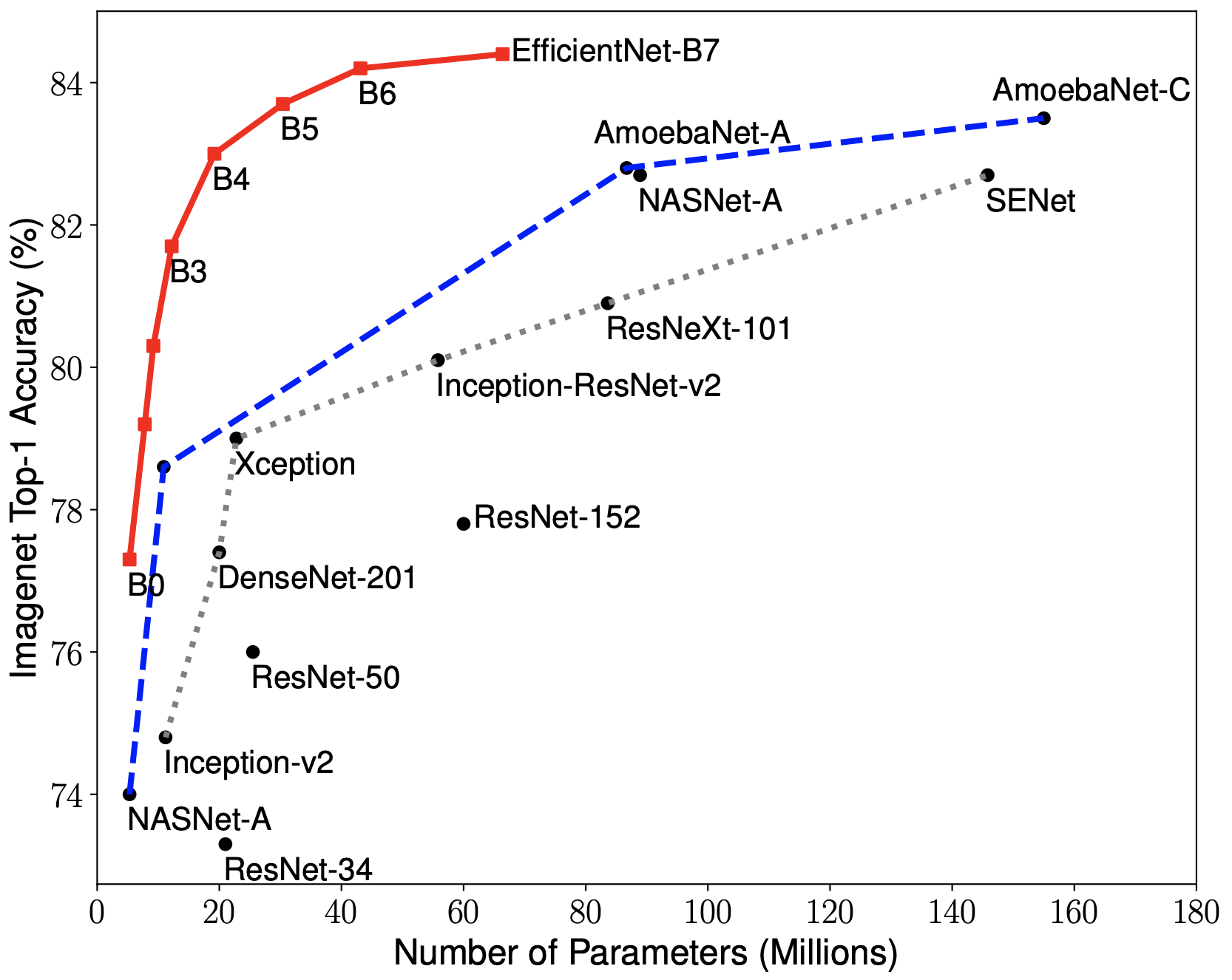","metadata":{}},{"cell_type":"markdown","source":"## Table Of Contents","metadata":{}},{"cell_type":"markdown","source":"- [Dependencies](#1)\n- [Preparation](#2)\n- [Metric (Quadratic Weighted Kappa)](#3)\n- [EDA (Exploratory Data Analysis)](#4)\n- [Preprocessing](#5)\n- [Modeling (EfficientNetB5)](#6)\n- [Evaluation](#7)\n- [Submission](#8)","metadata":{}},{"cell_type":"markdown","source":"## Dependencies ","metadata":{}},{"cell_type":"code","source":"import os\nimport sys\n\n# Standard dependencies\nimport cv2\nimport time\nimport scipy as sp\nimport numpy as np\nimport random as rn\nimport pandas as pd\nfrom tqdm import tqdm\nfrom PIL import Image\nfrom functools import partial\nimport matplotlib.pyplot as plt\n\n# Machine Learning\nimport tensorflow as tf\nimport keras\nfrom keras import initializers\nfrom keras import regularizers\nfrom keras import constraints\nfrom keras import backend as K\nfrom keras.activations import elu\nfrom keras.optimizers import Adam\nfrom keras.models import Sequential\nfrom keras.engine import Layer, InputSpec\nfrom keras.utils.generic_utils import get_custom_objects\nfrom keras.callbacks import Callback, EarlyStopping, ReduceLROnPlateau\nfrom keras.layers import Dense, Conv2D, Flatten, GlobalAveragePooling2D, Dropout\nfrom keras.preprocessing.image import ImageDataGenerator\nfrom sklearn.metrics import cohen_kappa_score\n\n# Path specifications\nKAGGLE_DIR = '../input/aptos2019-blindness-detection/'\nTRAIN_DF_PATH = KAGGLE_DIR + \"train.csv\"\nTEST_DF_PATH = KAGGLE_DIR + 'test.csv'\nTRAIN_IMG_PATH = KAGGLE_DIR + \"train_images/\"\nTEST_IMG_PATH = KAGGLE_DIR + 'test_images/'\n\n# Specify title of our final model\nSAVED_MODEL_NAME = 'effnet_b{}_model.h5'.format(EFFNET)\n\n# Set seed for reproducability\nseed = 1234\nrn.seed(seed)\nnp.random.seed(seed)\ntf.set_random_seed(seed)\nos.environ['PYTHONHASHSEED'] = str(seed)\n\n# For keeping time. GPU limit for this competition is set to ± 9 hours.\nt_start = time.time()","metadata":{"_kg_hide-input":true,"_kg_hide-output":true,"collapsed":true,"jupyter":{"outputs_hidden":true}},"execution_count":null,"outputs":[]},{"cell_type":"markdown","source":"Used wrapper to get the EfficientNet architecture in one line of code using [reference](https://github.com/qubvel/efficientnet). \n\n### Flow of Code:\n\n- Specify the input shape and create the model without the top (the final Dense layer). \n- Then we load in the weights for EfficientNet model.\n- we will use the [RAdam optimizer](https://arxiv.org/pdf/1908.03265v1.pdf) since it often yields better convergence than Vanilla Adam. ","metadata":{}},{"cell_type":"code","source":"!pip install ../input/efficientnet100\n!pip install ../input/kerasradam/\n!pip install ../input/kerascontrib/\n!pip install ../input/ipythonautotime/\n%load_ext autotime","metadata":{"_kg_hide-input":false,"_kg_hide-output":true,"collapsed":true,"jupyter":{"outputs_hidden":true}},"execution_count":null,"outputs":[]},{"cell_type":"code","source":"exec('from efficientnet.keras import EfficientNetB{} as EfficientNet'.format(EFFNET))\n\nfrom keras_radam import RAdam\nfrom keras_contrib.layers import GroupNormalization\n\nfrom sklearn.metrics import accuracy_score","metadata":{"_kg_hide-input":true,"_kg_hide-output":true,"collapsed":true,"jupyter":{"outputs_hidden":true}},"execution_count":null,"outputs":[]},{"cell_type":"markdown","source":"## Preparation ","metadata":{}},{"cell_type":"code","source":"TRAIN_TEST_RATIO = 1 - (70 + 15) / (70 + 15 + 15)\nTRAIN_VAL_RATIO = 1 - 70 / (70 + 15)","metadata":{"_kg_hide-output":true,"collapsed":true,"jupyter":{"outputs_hidden":true}},"execution_count":null,"outputs":[]},{"cell_type":"code","source":"# display train_df.head()\nprint(\"Image IDs and Labels (TRAIN)\")\ntrain_df = pd.read_csv(TRAIN_DF_PATH).sample(frac = 1, \n random_state = seed)\n\n# Add extension to id_code\ntrain_df['id_code'] = train_df['id_code'] + \".png\"\nprint(f\"Training images: { train_df.shape[0] }\")\n\n# display(test_df.head())\nprint(\"Image IDs (TEST)\")\ntest_df = pd.read_csv(TEST_DF_PATH) # .sample(frac=1, random_state=seed)\n\n# Add extension to id_code\ntest_df['id_code'] = test_df['id_code'] + \".png\"\ntest_df = test_df.rename(columns = { 'diagnosis': 'label' })\nprint(f\"Testing Images: { test_df.shape[0] }\")","metadata":{"_kg_hide-input":true,"collapsed":true,"jupyter":{"outputs_hidden":true}},"execution_count":null,"outputs":[]},{"cell_type":"markdown","source":"The original image size from the [EfficientNet paper](https://arxiv.org/pdf/1905.11946.pdf) for EfficientNetB5 is 456x456x3. We are however not bound by this and can use a smaller size if we want. The original image sizes used for every version of EfficientNet are:\n\n- EfficientNetB0 - (224, 224, 3)\n- EfficientNetB1 - (240, 240, 3)\n- EfficientNetB2 - (260, 260, 3)\n- EfficientNetB3 - (300, 300, 3)\n- EfficientNetB4 - (380, 380, 3)\n- **EfficientNetB5 - (456, 456, 3)**\n- EfficientNetB6 - (528, 528, 3)\n- EfficientNetB7 - (600, 600, 3)\n","metadata":{}},{"cell_type":"code","source":"# Specify image size\neffnet_to_img_size = dict(enumerate(\n [(224, 224), (240, 240), (260, 260), (300, 300), (380, 380), (456, 456), (528, 528), (600, 600)]\n))\nIMG_WIDTH, IMG_HEIGHT = effnet_to_img_size[EFFNET]\nCHANNELS = 3\n\n# Specify number of epochs\neffnet_to_nb_epochs = dict(enumerate([30, 30, 30, 30, 30, 25, 20, 15]))\nEPOCHS = effnet_to_nb_epochs[EFFNET]","metadata":{"_kg_hide-output":true,"collapsed":true,"jupyter":{"outputs_hidden":true}},"execution_count":null,"outputs":[]},{"cell_type":"markdown","source":"## Metric (Quadratic Weighted Kappa) ","metadata":{}},{"cell_type":"markdown","source":"The metric that is used for this kernel is Quadratic Weighted Kappa (QWK), which is evaluated using the formula:\n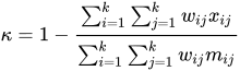","metadata":{}},{"cell_type":"code","source":"def get_preds_and_labels(model, generator):\n \"\"\"\n Get predictions and labels from the generator\n \n :param model: A Keras model object\n :param generator: A Keras ImageDataGenerator object\n \n :return: A tuple with two Numpy Arrays. One containing the predictions\n and one containing the labels\n \"\"\"\n preds = []\n labels = []\n for _ in range(int(np.ceil(generator.samples / BATCH_SIZE))):\n x, y = next(generator)\n preds.append(model.predict(x))\n labels.append(y)\n \n # Flatten list of numpy arrays\n return np.concatenate(preds).ravel(), np.concatenate(labels).ravel().astype(int)","metadata":{"_kg_hide-input":true,"_kg_hide-output":true,"collapsed":true,"jupyter":{"outputs_hidden":true}},"execution_count":null,"outputs":[]},{"cell_type":"code","source":"class Metrics(Callback):\n \"\"\"\n A custom Keras callback for saving the best model\n according to the Quadratic Weighted Kappa (QWK) metric\n \"\"\"\n def on_train_begin(self, logs={}):\n \"\"\"\n Initialize list of QWK scores on validation data\n \"\"\"\n self.val_kappas = []\n\n def on_epoch_end(self, epoch, logs={}):\n \"\"\"\n Gets QWK score on the validation data\n \n :param epoch: The current epoch number\n \"\"\"\n # Get predictions and convert to integers\n y_pred, labels = get_preds_and_labels(model, val_generator)\n y_pred = np.rint(y_pred).astype(np.uint8).clip(0, 4)\n \n # We can use sklearns implementation of QWK straight out of the box\n # as long as we specify weights as 'quadratic'\n _val_kappa = cohen_kappa_score(labels, y_pred, weights='quadratic')\n self.val_kappas.append(_val_kappa)\n print(f\"val_kappa: { round(_val_kappa, 4) }\")\n if _val_kappa == max(self.val_kappas):\n print(\"Validation Kappa has improved. Saving model.\")\n self.model.save(SAVED_MODEL_NAME)\n return","metadata":{"_kg_hide-input":true,"_kg_hide-output":true,"collapsed":true,"jupyter":{"outputs_hidden":true}},"execution_count":null,"outputs":[]},{"cell_type":"markdown","source":"## EDA (Exploratory Data Analysis) ","metadata":{}},{"cell_type":"markdown","source":"For EDA on the image dataset we examine the label distribution, the images before preprocessing and the images after preprocessing. Through examining these three aspects we can get a good sense of the problem. Note that the distribution on the test set can still vary wildly from the training data.","metadata":{}},{"cell_type":"code","source":"# Label distribution\ntrain_df['diagnosis'].value_counts().sort_index().plot(kind = \"bar\", \n figsize = (12, 5), \n rot = 0)\nplt.title(\"Label Distribution (Training Set)\", \n weight = 'bold', \n fontsize = 18)\nplt.xticks(fontsize = 15)\nplt.yticks(fontsize = 15)\nplt.xlabel(\"Label\", fontsize = 17)\nplt.ylabel(\"Frequency\", fontsize = 17);","metadata":{"_kg_hide-input":true,"collapsed":true,"jupyter":{"outputs_hidden":true}},"execution_count":null,"outputs":[]},{"cell_type":"markdown","source":"We will visualize a random image from every label to get a general sense of the distinctive features that seperate the classes. We will take this into account and try to enhance these features in our preprocessing. For these images there some to be increasingly more spots and stains on the retina as diabetic retinopathy worsens.","metadata":{}},{"cell_type":"code","source":"# Example from every label\nfig, ax = plt.subplots(1, 5, figsize = (15, 6))\nfor i in range(5):\n sample = train_df[train_df['diagnosis'] == i].sample(1)\n image_name = sample['id_code'].item()\n X = cv2.imread(f\"{ TRAIN_IMG_PATH } { image_name }\")\n ax[i].set_title(f\"Image: { image_name }\\n Label = { sample['diagnosis'].item() }\", \n weight = 'bold', fontsize = 10)\n ax[i].axis('off')\n ax[i].imshow(X);","metadata":{"_kg_hide-input":true,"collapsed":true,"jupyter":{"outputs_hidden":true}},"execution_count":null,"outputs":[]},{"cell_type":"markdown","source":"## Preprocessing ","metadata":{}},{"cell_type":"markdown","source":"Here we will use the auto-cropping method with three steps:\n1. input the image\n2. applying the mask\n3. resizing the image\n4. Adding gaussian noise to increase robustness","metadata":{}},{"cell_type":"code","source":"def crop_image_from_gray(img, tol = 7):\n \"\"\"\n Applies masks to the orignal image and returns the a preprocessed image with 3 channels\n \n :param img: A NumPy Array that will be cropped\n :param tol: The tolerance used for masking\n \n :return: A NumPy array containing the cropped image\n \"\"\"\n # If for some reason we only have two channels\n if img.ndim == 2:\n mask = img > tol\n return img[np.ix_(mask.any(1),mask.any(0))]\n \n # If we have a normal RGB images\n elif img.ndim == 3:\n gray_img = cv2.cvtColor(img, cv2.COLOR_RGB2GRAY)\n mask = gray_img > tol\n \n check_shape = img[:, :, 0][np.ix_(mask.any(1), mask.any(0))].shape[0]\n \n # image is too dark so that we crop out everything,\n if (check_shape == 0):\n # return original image\n return img \n else:\n img1 = img[:, :, 0][np.ix_(mask.any(1), mask.any(0))]\n img2 = img[:, :, 1][np.ix_(mask.any(1), mask.any(0))]\n img3 = img[:, :, 2][np.ix_(mask.any(1), mask.any(0))]\n img = np.stack([img1, img2, img3], axis = -1)\n return img\n\ndef preprocess_image(image, sigmaX = 10):\n \"\"\"\n :param img: A NumPy Array that will be cropped\n :param sigmaX: Value used for add GaussianBlur to the image\n \n :return: A NumPy array containing the preprocessed image\n \"\"\"\n image = cv2.cvtColor(image, cv2.COLOR_BGR2RGB)\n image = crop_image_from_gray(image)\n image = cv2.resize(image, (IMG_WIDTH, IMG_HEIGHT))\n # image = cv2.addWeighted (image,4, cv2.GaussianBlur(image, (0,0) ,sigmaX), -4, 128)\n return image","metadata":{"_kg_hide-input":true,"_kg_hide-output":true,"collapsed":true,"jupyter":{"outputs_hidden":true}},"execution_count":null,"outputs":[]},{"cell_type":"markdown","source":"After preprocessing we have managed to enhance the distinctive features in the images. This will increase performance when we train our EfficientNet model.","metadata":{}},{"cell_type":"code","source":"# Example of preprocessed images from every label\nfig, ax = plt.subplots(1, 5, figsize=(15, 6))\nfor i in range(5):\n sample = train_df[train_df['diagnosis'] == i].sample(1)\n image_name = sample['id_code'].item()\n X = preprocess_image(cv2.imread(f\"{ TRAIN_IMG_PATH } { image_name }\"))\n ax[i].set_title(f\"Image: { image_name }\\n Label = { sample['diagnosis'].item() }\", \n weight = 'bold', fontsize = 10)\n ax[i].axis('off')\n ax[i].imshow(X);","metadata":{"_kg_hide-input":true,"collapsed":true,"jupyter":{"outputs_hidden":true}},"execution_count":null,"outputs":[]},{"cell_type":"code","source":"# Labels for training data\ny_labels = train_df['diagnosis'].values","metadata":{"_kg_hide-output":true,"collapsed":true,"jupyter":{"outputs_hidden":true}},"execution_count":null,"outputs":[]},{"cell_type":"markdown","source":"## Modeling (EfficientNetB5) ","metadata":{}},{"cell_type":"markdown","source":"Since we are not provided with that much data (3662 images), we will augment the data to make the model more robust. We will rotate the data on any angle. Also, we will flip the data both horizontally and vertically. Lastly, we will divide the data by 128 for normalization.","metadata":{}},{"cell_type":"code","source":"# We use a small batch size so we can handle large images easily\nBATCH_SIZE = 4\n\n# Add Image augmentation to our generator\ntrain_datagen = ImageDataGenerator(rotation_range = 360,\n horizontal_flip = True,\n vertical_flip = True,\n validation_split = TRAIN_VAL_RATIO,\n preprocessing_function = preprocess_image, \n rescale = 1 / 255.)\n\n# Use the dataframe to define train and validation generators\ntrain_generator = train_datagen.flow_from_dataframe(train_df, \n x_col = 'id_code', \n y_col = 'diagnosis',\n directory = TRAIN_IMG_PATH,\n target_size = (IMG_WIDTH, IMG_HEIGHT),\n batch_size = BATCH_SIZE,\n class_mode = 'other', \n subset = 'training',\n seed = seed)\n\nval_generator = train_datagen.flow_from_dataframe(train_df, \n x_col = 'id_code', \n y_col = 'diagnosis',\n directory = TRAIN_IMG_PATH,\n target_size = (IMG_WIDTH, IMG_HEIGHT),\n batch_size = BATCH_SIZE,\n class_mode = 'other',\n subset = 'validation',\n seed = seed)","metadata":{"_kg_hide-output":true,"collapsed":true,"jupyter":{"outputs_hidden":true}},"execution_count":null,"outputs":[]},{"cell_type":"code","source":"# Load in EfficientNetB5\neffnet = EfficientNet(weights = 'imagenet',\n include_top = False,\n input_shape=(IMG_WIDTH, IMG_HEIGHT, CHANNELS))\neffnet.load_weights(\n '../input/efficientnet-weights-for-keras/advprop/notop/efficientnet-b{}_weights_imagenet_1000_advprop_notop.h5'.format(\n EFFNET\n )\n)","metadata":{"_kg_hide-output":true,"collapsed":true,"jupyter":{"outputs_hidden":true}},"execution_count":null,"outputs":[]},{"cell_type":"code","source":"# Replace all Batch Normalization layers by Group Normalization layers\nfor i, layer in enumerate(effnet.layers):\n if \"batch_normalization\" in layer.name:\n effnet.layers[i] = GroupNormalization(groups=32, axis=-1, epsilon=0.00001)","metadata":{"_kg_hide-output":true,"collapsed":true,"jupyter":{"outputs_hidden":true}},"execution_count":null,"outputs":[]},{"cell_type":"code","source":"def build_model():\n \"\"\"\n A custom implementation of EfficientNetB5\n for the APTOS 2019 competition\n (Regression)\n \"\"\"\n model = Sequential()\n model.add(effnet)\n model.add(GlobalAveragePooling2D())\n model.add(Dropout(0.5))\n model.add(Dense(5, activation=elu))\n model.add(Dense(1, activation=\"linear\"))\n model.compile(loss='mse',\n optimizer=RAdam(learning_rate=0.00005), \n metrics=['mse', 'acc'])\n print(model.summary())\n return model\n\n# Initialize model\nmodel = build_model()","metadata":{"_kg_hide-output":false,"collapsed":true,"jupyter":{"outputs_hidden":true}},"execution_count":null,"outputs":[]},{"cell_type":"markdown","source":"We train all layers in the network. This is the traditional transfer learning approach were we can optimize and model for almost any image content. Since the pre-trained model was trained on [ImageNet](http://www.image-net.org/) and not on medical images, there are some limitations to this approach for out challenge.\n\nAfter each epoch we save the model if it is better than the previous one, according to the Quadratic Weighted Kappa score on the validation set. We also stop training if the MSE on the validation set doesn't go down for 4 epochs. This way we can counter overfitting.\n\nAnother option we could use is to directly use Quadratic Weighted Kappa as a loss function. Feel free to experiment with this. An implementation of a [QWK loss function for Tensorflow/Keras can be found in this Kaggle kernel](https://www.kaggle.com/christofhenkel/weighted-kappa-loss-for-keras-tensorflow).","metadata":{}},{"cell_type":"code","source":"# For tracking Quadratic Weighted Kappa score\nkappa_metrics = Metrics()\n\n# Monitor MSE to avoid overfitting and save best model\nes = EarlyStopping(monitor = 'val_loss', mode = 'auto', verbose = 1, patience = EPOCHS // 2)\nrlr = ReduceLROnPlateau(monitor = 'val_loss', \n factor = 0.5, \n patience = EPOCHS // 4, \n verbose = 1, \n mode = 'auto', \n min_delta = 0.0001)\n\n# Begin training\nmodel.fit_generator(train_generator,\n steps_per_epoch = train_generator.samples // BATCH_SIZE,\n epochs = EPOCHS,\n validation_data = val_generator,\n validation_steps = val_generator.samples // BATCH_SIZE,\n callbacks = [kappa_metrics, es, rlr])","metadata":{"_kg_hide-output":true,"collapsed":true,"jupyter":{"outputs_hidden":true}},"execution_count":null,"outputs":[]},{"cell_type":"code","source":"# Visualize mse\nhistory_df = pd.DataFrame(model.history.history)\nhistory_df[['loss', 'val_loss']].plot(figsize = (12, 5))\nplt.title(\"Loss (MSE)\", fontsize = 16, weight = 'bold')\nplt.xlabel(\"Epoch\")\nplt.ylabel(\"Loss (MSE)\")\nhistory_df[['acc', 'val_acc']].plot(figsize = (12, 5))\nplt.title(\"Accuracy\", fontsize = 16, weight = 'bold')\nplt.xlabel(\"Epoch\")\nplt.ylabel(\"% Accuracy\");","metadata":{"_kg_hide-input":true},"execution_count":null,"outputs":[]},{"cell_type":"markdown","source":"## Evaluation ","metadata":{}},{"cell_type":"code","source":"# Load best weights according to MSE\nmodel.load_weights(SAVED_MODEL_NAME)","metadata":{},"execution_count":null,"outputs":[]},{"cell_type":"markdown","source":"To evaluate our performance we predict values from the generator and round them of to the nearest integer to get valid predictions. After that we calculate the Quadratic Weighted Kappa score on the training set and the validation set.","metadata":{}},{"cell_type":"code","source":"from sklearn.model_selection import train_test_split\nfrom sklearn.metrics import confusion_matrix\nfrom sklearn.utils.multiclass import unique_labels\n\ndef plot_confusion_matrix(y_true, y_pred, classes,\n normalize=False,\n title=None,\n cmap=plt.cm.Blues):\n \"\"\"\n This function prints and plots the confusion matrix.\n Normalization can be applied by setting `normalize=True`.\n \"\"\"\n if not title:\n if normalize:\n title = 'Normalized confusion matrix'\n else:\n title = 'Confusion matrix, without normalization'\n\n # Compute confusion matrix\n cm = confusion_matrix(y_true, y_pred)\n \n # Only use the labels that appear in the data\n classes = classes[unique_labels(y_true, y_pred)]\n if normalize:\n cm = cm.astype('float') / cm.sum(axis = 1)[:, np.newaxis]\n print(\"Normalized confusion matrix\")\n else:\n print('Confusion matrix, without normalization')\n\n print(cm)\n\n fig, ax = plt.subplots()\n im = ax.imshow(cm, interpolation = 'nearest', cmap = cmap)\n ax.figure.colorbar(im, ax = ax)\n ax.set(xticks = np.arange(cm.shape[1]), yticks = np.arange(cm.shape[0]),\n xticklabels = classes, yticklabels = classes,\n title = title,\n ylabel = 'True label', xlabel = 'Predicted label')\n\n # Rotate the tick labels and set their alignment.\n plt.setp(ax.get_xticklabels(), rotation = 45, ha = \"right\",\n rotation_mode = \"anchor\")\n\n # Loop over data dimensions and create text annotations.\n fmt = '.2f' if normalize else 'd'\n thresh = cm.max() / 2.\n for i in range(cm.shape[0]):\n for j in range(cm.shape[1]):\n ax.text(j, i, format(cm[i, j], fmt),\n ha = \"center\", va = \"center\",\n color = \"white\" if cm[i, j] > thresh else \"black\")\n fig.tight_layout()\n return ax\n\nnp.set_printoptions(precision = 2)","metadata":{"_kg_hide-input":true,"_kg_hide-output":true,"collapsed":true,"jupyter":{"outputs_hidden":true}},"execution_count":null,"outputs":[]},{"cell_type":"code","source":"class OptimizedRounder(object):\n \"\"\"\n An optimizer for rounding thresholds to maximize Quadratic Weighted Kappa score\n \"\"\"\n def __init__(self):\n self.coef_ = 0\n\n def _kappa_loss(self, coef, X, y):\n \"\"\"\n Get loss according to raw predictions using current coefficients\n \n :param coef: A list of coefficients that will be used for rounding\n :param X: The raw predictions\n :param y: The ground truth labels\n \"\"\"\n X_p = np.copy(X)\n for i, pred in enumerate(X_p):\n if pred < coef[0]:\n X_p[i] = 0\n elif pred >= coef[0] and pred < coef[1]:\n X_p[i] = 1\n elif pred >= coef[1] and pred < coef[2]:\n X_p[i] = 2\n elif pred >= coef[2] and pred < coef[3]:\n X_p[i] = 3\n else:\n X_p[i] = 4\n\n ll = cohen_kappa_score(y, X_p, weights='quadratic')\n return -ll\n\n def fit(self, X, y):\n \"\"\"\n Optimize rounding thresholds\n \n :param X: The raw predictions\n :param y: The ground truth labels\n \"\"\"\n loss_partial = partial(self._kappa_loss, X = X, y = y)\n initial_coef = [0.5, 1.5, 2.5, 3.5]\n self.coef_ = sp.optimize.minimize(loss_partial, initial_coef, method = 'nelder-mead')\n\n def predict(self, X, coef):\n \"\"\"\n Make predictions with specified thresholds\n \n :param X: The raw predictions\n :param coef: A list of coefficients that will be used for rounding\n \"\"\"\n X_p = np.copy(X)\n for i, pred in enumerate(X_p):\n if pred < coef[0]:\n X_p[i] = 0\n elif pred >= coef[0] and pred < coef[1]:\n X_p[i] = 1\n elif pred >= coef[1] and pred < coef[2]:\n X_p[i] = 2\n elif pred >= coef[2] and pred < coef[3]:\n X_p[i] = 3\n else:\n X_p[i] = 4\n return X_p.astype(int)\n\n def coefficients(self):\n \"\"\"\n Return the optimized coefficients\n \"\"\"\n return self.coef_['x']","metadata":{"_kg_hide-input":true,"_kg_hide-output":true},"execution_count":null,"outputs":[]},{"cell_type":"code","source":"# Optimize on validation data and evaluate again\ny_val_preds, val_labels = get_preds_and_labels(model, val_generator)\n\noptR = OptimizedRounder()\noptR.fit(y_val_preds, val_labels)\n\ncoefficients = optR.coefficients()\nopt_val_predictions = optR.predict(y_val_preds, coefficients)\nnew_val_score = cohen_kappa_score(val_labels, opt_val_predictions, weights = \"quadratic\")\nnew_acc_val_score = accuracy_score(val_labels, opt_val_predictions)","metadata":{},"execution_count":null,"outputs":[]},{"cell_type":"code","source":"print(f\"Optimized Thresholds:\\n{ coefficients }\\n\")\n\nprint(f\"The Validation Quadratic Weighted Kappa (QWK)\\n\\\nwith optimized rounding thresholds is: {round(new_val_score, 5)}\\n\")\n\nprint(f\"The Validation Accuracy\\n\\\nwith optimized rounding thresholds is: {round(new_acc_val_score, 5)}\\n\")","metadata":{"_kg_hide-input":true},"execution_count":null,"outputs":[]},{"cell_type":"code","source":"# Plot non-normalized confusion matrix\nplot_confusion_matrix(val_labels, opt_val_predictions, classes=np.array(['0', '1', '2', '3', '4']),\n title='Confusion matrix, without normalization')\nplt.show()","metadata":{},"execution_count":null,"outputs":[]},{"cell_type":"markdown","source":"## Predictions on Test set ","metadata":{}},{"cell_type":"markdown","source":"Since the test set is not that large we will not be using a generator for making the final predictions on the test set.","metadata":{}},{"cell_type":"code","source":"# Place holder for diagnosis column\ntest_df['diagnosis'] = np.zeros(test_df.shape[0]) \n\n# For preprocessing test images\ntest_generator = ImageDataGenerator(preprocessing_function = preprocess_image, rescale = 1 / 255.)\ntest_generator = test_generator.flow_from_dataframe(test_df, \n x_col = 'id_code', y_col = 'diagnosis',\n directory=TEST_IMG_PATH,\n target_size = (IMG_WIDTH, IMG_HEIGHT),\n batch_size = BATCH_SIZE,\n class_mode = 'other',\n shuffle = False,\n seed = seed)","metadata":{"_kg_hide-output":true,"collapsed":true,"jupyter":{"outputs_hidden":true}},"execution_count":null,"outputs":[]},{"cell_type":"code","source":"# Make final predictions, round predictions and save to csv\ny_test, _ = get_preds_and_labels(model, test_generator)\ny_test = optR.predict(y_test, coefficients).astype(np.uint8)\ntest_df['diagnosis'] = y_test\n\n# Remove .png from ids\ntest_df['id_code'] = test_df['id_code'].str.replace(r'.png$', '')\ntest_df.to_csv('submission.csv', index=False)","metadata":{"_kg_hide-input":false,"_kg_hide-output":true,"collapsed":true,"jupyter":{"outputs_hidden":true}},"execution_count":null,"outputs":[]},{"cell_type":"markdown","source":"checking the format and the distribution of the test predictions. ","metadata":{}},{"cell_type":"code","source":"# Check submission\nprint(\"Submission File\")\ndisplay(test_df.head())","metadata":{"_kg_hide-input":true,"collapsed":true,"jupyter":{"outputs_hidden":true}},"execution_count":null,"outputs":[]},{"cell_type":"code","source":"# Label distribution\ntrain_df['diagnosis'].value_counts().sort_index().plot(kind = \"bar\", \n figsize = (12, 5), \n rot = 0)\nplt.title(\"Label Distribution (Training Set)\", \n weight = 'bold', \n fontsize = 18)\nplt.xticks(fontsize = 15)\nplt.yticks(fontsize = 15)\nplt.xlabel(\"Label\", fontsize = 17)\nplt.ylabel(\"Frequency\", fontsize = 17)","metadata":{"_kg_hide-input":true,"collapsed":true,"jupyter":{"outputs_hidden":true}},"execution_count":null,"outputs":[]},{"cell_type":"code","source":"# Distribution of predictions\ntest_df['diagnosis'].value_counts().sort_index().plot(kind=\"bar\", \n figsize=(12,5), \n rot=0)\nplt.title(\"Label Distribution (Predictions)\", \n weight = 'bold', \n fontsize = 18)\nplt.xticks(fontsize = 15)\nplt.yticks(fontsize = 15)\nplt.xlabel(\"Label\", fontsize = 17)\nplt.ylabel(\"Frequency\", fontsize = 17)","metadata":{"_kg_hide-input":true,"collapsed":true,"jupyter":{"outputs_hidden":true}},"execution_count":null,"outputs":[]},{"cell_type":"code","source":"# Check kernels run-time\nt_finish = time.time()\ntotal_time = round((t_finish-t_start) / 3600, 4)\nprint('Kernel runtime = {} hours ({} minutes)'.format(total_time, int(total_time * 60)))","metadata":{"_kg_hide-input":true,"collapsed":true,"jupyter":{"outputs_hidden":true}},"execution_count":null,"outputs":[]}]}