 \n\n
\n\nHenry AI Labs
\n \n\n\n
 \n\n## 1.1 Description\n\n* **Current Methods** : Produce unreliable results, raising false alarms\n* **Data** : images acquired with ~ 50 different cameras and processed in different fashions\n\n## 1.2 Evaluation\n* submissions are evaluated on the *weighted AUC*\n* each region of the ROC curve is weighted according to these chosen parameters:\n * `tpr_thresholds = [0.0, 0.4, 1.0]`\n * `weights = [2, 1]`\n\n
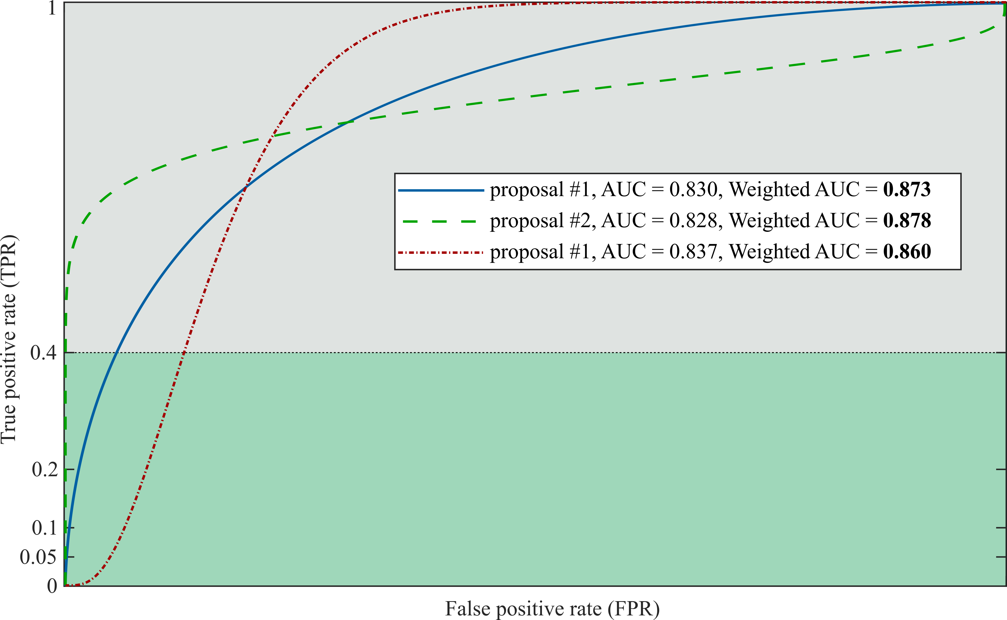 \n\n## 1.3 Sumbission file\nFor each Id (image) in the test set, you must provide a score that indicates *how likely this image contains hidden data*: the higher the score, the more it is assumed that image contains secret data.\n\n## 1.4 Data\n**Files**\n* `Cover/` contains 75k unaltered images meant for use in training.\n* `JMiPOD/` contains 75k examples of the JMiPOD algorithm applied to the cover images.\n* `JUNIWARD/` contains 75k examples of the JUNIWARD algorithm applied to the cover images.\n* `UERD/` contains 75k examples of the UERD algorithm applied to the cover images.\n* `Test/` contains 5k test set images. These are the images for which you are predicting.\n* `sample_submission.csv` contains an example submission in the correct format.","execution_count":null},{"metadata":{},"cell_type":"markdown","source":"# 2. Libraries 📚","execution_count":null},{"metadata":{"_kg_hide-output":true,"trusted":true,"_kg_hide-input":true},"cell_type":"code","source":"!pip install stegano # steganalysis library\n!pip install -q efficientnet_pytorch # Convolutional Neural Net from Google Research","execution_count":null,"outputs":[]},{"metadata":{"trusted":true,"_kg_hide-output":true,"_kg_hide-input":true},"cell_type":"code","source":"import stegano\nfrom stegano import lsb\n\n# System\nimport cv2\nimport os, os.path\nfrom PIL import Image # from RBG to YCbCr\n\n# Basics\nimport pandas as pd\nimport numpy as np\nfrom numpy import pi # for DCT\nfrom numpy import r_ # for DCT\nimport scipy # for cosine similarity\nfrom scipy import fftpack # for DCT\nimport random\nimport seaborn as sns\nimport matplotlib.pyplot as plt\nimport matplotlib.image as mpimg # to check images\n%matplotlib inline\nfrom tqdm.notebook import tqdm # beautiful progression bar\n\n# SKlearn\nfrom sklearn.model_selection import KFold\nfrom sklearn import metrics\n\n# PyTorch\nimport torch\nimport torch.nn as nn\nimport torch.optim as optim\nfrom torch import FloatTensor, LongTensor\nfrom torch.utils.data import Dataset, DataLoader\nfrom torch.optim.lr_scheduler import ReduceLROnPlateau\nimport torch.nn.functional as F\n\n# Data Augmentation for Image Preprocessing\nfrom albumentations import (ToFloat, Normalize, VerticalFlip, HorizontalFlip, Compose, Resize,\n RandomBrightness, RandomContrast, HueSaturationValue, Blur, GaussNoise)\nfrom albumentations.pytorch import ToTensorV2, ToTensor\nfrom efficientnet_pytorch import EfficientNet\nfrom torchvision.models import resnet34\n\nimport warnings\nwarnings.filterwarnings(\"ignore\")","execution_count":null,"outputs":[]},{"metadata":{"trusted":true,"_kg_hide-input":true,"_kg_hide-output":true},"cell_type":"code","source":"print(list(os.listdir(\"../input/v2-effnet-epoch-6-auc-08023\")))","execution_count":null,"outputs":[]},{"metadata":{},"cell_type":"markdown","source":"# 3. Example: Stegano Library\n\n**Images encoded data**: Usually images have 3 channels (RGB), composed by pixels, which *describe* the image (the colors).\n
 \n\n> [Stegano package documentation](https://buildmedia.readthedocs.org/media/pdf/stegano/latest/stegano.pdf) : this package hides the *hidden information* in the *least significant bits* of the image. These bits have the property of being very random (white noise), so they don't *fire* when some change is applied to them. ","execution_count":null},{"metadata":{"trusted":true},"cell_type":"code","source":"# Create a new image with secret message\nmsg_to_hide = \"Message encoded blue cats from Mars are coming to enslave us all be aware!!!!!!\"\nsecret = lsb.hide(\"../input/suki-image/capture27.png\", \n msg_to_hide, \n auto_convert_rgb=True)\nsecret.save(\"./SukiSecret.png\")\n\n# Reveal the hidden message\nprint(lsb.reveal(\"./SukiSecret.png\"))\n\n# See the 2 images side by side (no apparent difference, but WE KNOW the text is there.)\nf, ax = plt.subplots(1, 2, figsize=(14,5))\n \noriginal = mpimg.imread('../input/suki-image/capture27.png')\noriginal_plot = ax[0].imshow(original)\n\naltered = mpimg.imread('./SukiSecret.png')\naltered_plot = ax[1].imshow(altered)","execution_count":null,"outputs":[]},{"metadata":{},"cell_type":"markdown","source":"### Checking Similarity 🌜🌛\nWe can check how similar are the images by substracting one matrix from the other. \n\nLet's check the **similarity** of the abote 2 images, to see if there is any hidden information in the altered image:","execution_count":null},{"metadata":{"trusted":true},"cell_type":"code","source":"# From image to array \n# (vectorize the matrix to be able to feed it to the cosine function)\noriginal_vector = np.array(original).flatten()\naltered_vector = np.array(altered).flatten()\n\nprint('Original shape:', original_vector.shape, '\\n' +\n 'Altered shape:', altered_vector.shape)\n\n\n# Distance between the original image and itself (should be 0, because they are identical)\ndist1 = np.sum(original_vector - original_vector)\nprint('Dist1:', dist1)\n\n# Distance between the original image and altered image\ndist2 = np.sum(original_vector - altered_vector)\nprint('Dist2:', dist2)","execution_count":null,"outputs":[]},{"metadata":{},"cell_type":"markdown","source":"# 4. Alaska2 Images - EDA\n\n## 4.1 Read in the data\nThere are 75k files in Cover, JMiPOD, JUNIWARD and UERD and 5k files in Test. We can't read the image arrays all at once, because the available RAM is not enough to perform this task.","execution_count":null},{"metadata":{"trusted":true,"_kg_hide-input":true},"cell_type":"code","source":"# ---- STATICS ----\nbase_path = '../input/alaska2-image-steganalysis'\n\ndef read_images_path(dir_name='Cover', test = False):\n '''series_name: 0001.jpg, 0002.jpg etc.\n series_paths: is the complete path to a certain image.'''\n \n # Get name of the files\n series_name = pd.Series(os.listdir(base_path + '/' + dir_name))\n if test:\n series_name = pd.Series(os.listdir(base_path + '/' + 'Test'))\n \n # Create the entire path\n series_paths = pd.Series(base_path + '/' + dir_name + '/' + series_name)\n \n return series_paths","execution_count":null,"outputs":[]},{"metadata":{"trusted":true},"cell_type":"code","source":"# Read in the data\ncover_paths = read_images_path('Cover', False)\njmipod_paths = read_images_path('JMiPOD', False)\njuniward_paths = read_images_path('JUNIWARD', False)\nuerd_paths = read_images_path('UERD', False)\ntest_paths = read_images_path('Test', True)","execution_count":null,"outputs":[]},{"metadata":{},"cell_type":"markdown","source":"### Show some Images","execution_count":null},{"metadata":{"trusted":true,"_kg_hide-input":true},"cell_type":"code","source":"def show15(title = \"Default\"):\n '''Shows n amount of images in the data'''\n plt.figure(figsize=(16,9))\n plt.suptitle(title, fontsize = 16)\n \n for k, path in enumerate(cover_paths[:15]):\n cover = mpimg.imread(path)\n \n plt.subplot(3, 5, k+1)\n plt.imshow(cover)\n plt.axis('off')","execution_count":null,"outputs":[]},{"metadata":{"trusted":true},"cell_type":"code","source":"show15(title = \"15 Original Images\")","execution_count":null,"outputs":[]},{"metadata":{},"cell_type":"markdown","source":"### Images shape, size, data type\n* all images are 512 x 512 x 3\n* all images are of size 786,432 \n* all images are uint8 type","execution_count":null},{"metadata":{"trusted":true},"cell_type":"code","source":"image_sample = mpimg.imread(cover_paths[0])\n\nprint('Image sample shape:', image_sample.shape)\nprint('Image sample size:', image_sample.size)\nprint('Image sample data type:', image_sample.dtype)","execution_count":null,"outputs":[]},{"metadata":{},"cell_type":"markdown","source":"## 4.2 Algorithms\nThere are 3 main different algorithms applied to the original image and used to encode information into it:\n* JMiPOD \n* JUNIWARD\n* UERD\n\n> All images have the corresponding encoding at the same name.","execution_count":null},{"metadata":{"trusted":true,"_kg_hide-input":true},"cell_type":"code","source":"def show_images_alg(n = 3, title=\"Default\"):\n '''Returns a plot of the original Image and Encoded ones.\n n: number of images to display'''\n \n f, ax = plt.subplots(n, 4, figsize=(16, 7))\n plt.suptitle(title, fontsize = 16)\n \n\n for index in range(n):\n cover = mpimg.imread(cover_paths[index])\n ipod = mpimg.imread(jmipod_paths[index])\n juni = mpimg.imread(juniward_paths[index])\n uerd = mpimg.imread(uerd_paths[index])\n\n # Plot\n ax[index, 0].imshow(cover)\n ax[index, 1].imshow(ipod)\n ax[index, 2].imshow(juni)\n ax[index, 3].imshow(uerd)\n \n # Add titles\n if index == 0:\n ax[index, 0].set_title('Original', fontsize=12)\n ax[index, 1].set_title('IPod', fontsize=12)\n ax[index, 2].set_title('Juni', fontsize=12)\n ax[index, 3].set_title('Uerd', fontsize=12)","execution_count":null,"outputs":[]},{"metadata":{"trusted":true},"cell_type":"code","source":"show_images_alg(n = 3, title = \"Algorithm Difference\")","execution_count":null,"outputs":[]},{"metadata":{},"cell_type":"markdown","source":"# 5. JPEG Images: Where is the information?\n\n* [Inspo and Understanding here](https://www.kaggle.com/tanulsingh077/steganalysis-complete-understanding-and-model)\n* [From Image to JPEG here](https://www.graphicsmill.com/docs/gm5/UnderstandingofJPEGEncodingParameters.htm)\n\n
 \n\n\n### Hiding information\n1. In the YCbCr channels: this is an old approach and can be easily found (as we saw in the Suki example)\n2. DCT Coefficients of the YCbCr channels: the payload (secret information) is randomly distributed\n\n> Either YCbCr or DCT Coeff can be used as **inputs** to the neural net\n\n## 5.1 Visualize YCbCr Channels:","execution_count":null},{"metadata":{"trusted":true,"_kg_hide-input":true},"cell_type":"code","source":"def show_ycbcr_images(n = 3, title = \"Default\"):\n '''Shows n images as: original RGB, YCbCr and Y, Cb, Cr channels split'''\n \n # 4: original image, YCbCr image, Y, Cb, Cr (separate chanels)\n fig, ax = plt.subplots(n, 5, figsize=(16, 7))\n plt.suptitle(title, fontsize = 16)\n\n for index, path in enumerate(cover_paths[:n]):\n # Read in the original image and convert\n original_image = Image.open(path)\n ycbcr_image = original_image.convert('YCbCr')\n (y, cb, cr) = ycbcr_image.split()\n\n # Plot\n ax[index, 0].imshow(original_image)\n ax[index, 1].imshow(ycbcr_image)\n ax[index, 2].imshow(y)\n ax[index, 3].imshow(cb)\n ax[index, 4].imshow(cr)\n\n # Add Title\n if index==0:\n ax[index, 0].set_title('Original', fontsize=12)\n ax[index, 1].set_title('YCbCr', fontsize=12)\n ax[index, 2].set_title('Y', fontsize=12)\n ax[index, 3].set_title('Cb', fontsize=12)\n ax[index, 4].set_title('Cr', fontsize=12)","execution_count":null,"outputs":[]},{"metadata":{"trusted":true},"cell_type":"code","source":"show_ycbcr_images(n = 3, title = \"YCbCr Channels\")","execution_count":null,"outputs":[]},{"metadata":{},"cell_type":"markdown","source":"## 5.2 Visualize DCT Coefficients:\n\n### Discrete Cosine Transform Example\n* [finite sequence of data points in terms of a sum of cosine functions oscillating at different frequencies](https://en.wikipedia.org/wiki/Discrete_cosine_transform)\n* transformation tenchnique for data compression \n* uses *cosine* rather than *sine* (faster computation)\n\n> [The following code is completely taken from this page: JPEG DCT Demo](https://inst.eecs.berkeley.edu/~ee123/sp16/Sections/JPEG_DCT_Demo.html#Display-all-DCT-blocks)","execution_count":null},{"metadata":{"trusted":true,"_kg_hide-input":true},"cell_type":"code","source":"# Read in an Image Example\nimage = mpimg.imread(cover_paths[2])\n\nplt.figure(figsize = (6, 6))\nplt.imshow(image)\nplt.title('Original Image', fontsize=16)\nplt.axis('off');","execution_count":null,"outputs":[]},{"metadata":{},"cell_type":"markdown","source":"#### Create DCT Function:","execution_count":null},{"metadata":{"trusted":true,"_kg_hide-input":true},"cell_type":"code","source":"# Define 2D DCT\ndef dct2(a):\n # Return the Discrete Cosine Transform of arbitrary type sequence x.\n return fftpack.dct(fftpack.dct( a, axis=0, norm='ortho' ), axis=1, norm='ortho')\n\n# Perform a blockwise DCT\nimsize = image.shape\ndct = np.zeros(imsize)\n\n# Do 8x8 DCT on image (in-place)\nfor i in r_[:imsize[0]:8]:\n for j in r_[:imsize[1]:8]:\n dct[i:(i+8),j:(j+8)] = dct2( image[i:(i+8),j:(j+8)] )","execution_count":null,"outputs":[]},{"metadata":{},"cell_type":"markdown","source":"### Look at an 8x8 block: original vs DCT coeff","execution_count":null},{"metadata":{"_uuid":"d629ff2d2480ee46fbb7e2d37f6b5fab8052498a","_cell_guid":"79c7e3d0-c299-4dcb-8224-4455121ee9b0","trusted":true,"_kg_hide-input":true},"cell_type":"code","source":"# ---- STATICS ----\npos = 128 # can be changed\n\nfig, (ax1, ax2) = plt.subplots(1, 2, figsize=(14, 6))\n\n# Display original\nax1.imshow(image[pos:pos+8,pos:pos+8],cmap='gray')\nax1.set_title(\"An 8x8 block : Original Image\", fontsize=16)\n\n# Display the dct of that block\nax2.imshow(dct[pos:pos+8,pos:pos+8],cmap='gray',vmax= np.max(dct)*0.01,vmin = 0, extent=[0,pi,pi,0])\nax2.set_title(\"An 8x8 DCT block\", fontsize = 16);","execution_count":null,"outputs":[]},{"metadata":{},"cell_type":"markdown","source":"### Display ALL DCT blocks against the original image","execution_count":null},{"metadata":{"trusted":true,"_kg_hide-input":true},"cell_type":"code","source":"fig, (ax1, ax2) = plt.subplots(1, 2, figsize=(14, 6))\n\n# Original image\nax1.imshow(image);\nax1.set_title(\"Original Image\", fontsize = 16);\n\n# DCT Blocks\nax2.imshow(dct,cmap='gray',vmax = np.max(dct)*0.01,vmin = 0)\nax2.set_title(\"DCT blocks\", fontsize = 14);","execution_count":null,"outputs":[]},{"metadata":{},"cell_type":"markdown","source":"### Bonus: Threshold DCT Coefficients\n> Keeping only a percentage of the coefficients","execution_count":null},{"metadata":{"trusted":true,"_kg_hide-input":true},"cell_type":"code","source":"# Threshold\nthresh = 0.02\ndct_thresh = dct * (abs(dct) > (thresh*np.max(dct)))\n\n\nplt.figure(figsize=(14, 6))\nplt.imshow(dct_thresh, cmap='gray', vmax = np.max(dct)*0.01, vmin = 0)\nplt.title(\"Thresholded 8x8 DCTs of the image\", fontsize = 16)\n\npercent_nonzeros = np.sum( dct_thresh != 0.0 ) / (imsize[0]*imsize[1]*1.0)\nprint(\"Keeping only {}% of the DCT coefficients\".format(round(percent_nonzeros*100.0, 3)))","execution_count":null,"outputs":[]},{"metadata":{},"cell_type":"markdown","source":"
Note: Inspiration for this notebook is from Alaska2 CNN Multiclass Classifier
\n ","execution_count":null},{"metadata":{"trusted":true},"cell_type":"code","source":"# ----- STATICS -----\nsample_size = 256\nnum_classes = 4\n# -------------------\n\n# Read in Data\n\n# --- 10 classes ---\n# train_df = pd.read_csv('../input/alaska2trainvalsplit/alaska2_train_df.csv', \n# header=0, names=['Path', 'Label'], dtype = {'Label':np.int32})\n# valid_df = pd.read_csv('../input/alaska2trainvalsplit/alaska2_val_df.csv', \n# header=0, names=['Path', 'Label'], dtype = {'Label':np.int32})\n\n# --- 4 classes ---\ntrain_df = pd.read_csv('../input/alaska2-trainvalid-4-class-csv/alaska2_train_data_4classes.csv', \n header=0, names=['Path', 'Label'], dtype = {'Label':np.int32})\nvalid_df = pd.read_csv('../input/alaska2-trainvalid-4-class-csv/alaska2_valid_data_4classes.csv', \n header=0, names=['Path', 'Label'], dtype = {'Label':np.int32})\n\n# Sample out Data\ndef sample_data(dataframe, sample_size, num_classes, train=True):\n '''Sample same number of images for each label.'''\n if train:\n size = int(0.75 * sample_size)\n else:\n size = int(0.25 * sample_size)\n \n # Number of images in class\n no = int(np.floor(size/num_classes))\n labels = [i for i in range(num_classes)]\n new_data = pd.DataFrame()\n \n # For each label\n for label in labels:\n # Sample out data\n data = dataframe[dataframe['Label'] == label].sample(no, random_state=123)\n new_data = pd.concat([new_data, data], axis=0)\n \n return new_data","execution_count":null,"outputs":[]},{"metadata":{"trusted":true},"cell_type":"code","source":"# Sample out data\ntrain_df = sample_data(train_df, num_classes=num_classes, \n sample_size=sample_size, train=True).reset_index(drop=True)\nvalid_df = sample_data(valid_df, num_classes=num_classes, \n sample_size=sample_size, train=False).reset_index(drop=True)","execution_count":null,"outputs":[]},{"metadata":{},"cell_type":"markdown","source":"#### Check if the result is OK","execution_count":null},{"metadata":{"trusted":true},"cell_type":"code","source":"print('Train Data Size:', len(train_df), '\\n' +\n 'Valid Data Size:', len(valid_df), '\\n' +\n '----------------------', '\\n' +\n 'Total:', len(train_df) + len(valid_df))\n\nfig, (ax1, ax2) = plt.subplots(1, 2, figsize = (14, 5))\n\nsns.countplot(x = train_df['Label'], ax = ax1, palette = sns.color_palette(\"GnBu_d\", 10))\nsns.countplot(x = valid_df['Label'], ax = ax2, palette = sns.color_palette(\"YlOrRd\", 10))\n\nax1.set_title('Train Data', fontsize=16)\nax2.set_title('Valid Data', fontsize=16);","execution_count":null,"outputs":[]},{"metadata":{},"cell_type":"markdown","source":"# 2. PyTorch Dataset 🛠\n\n### Dataset Class\n[Link here with example and more explanations](https://pytorch.org/tutorials/beginner/data_loading_tutorial.html)\n\n`torch.utils.data.Dataset` is an abstract class representing a dataset. Your custom dataset should inherit `Dataset` and override the following methods:\n* `__len__` so that len(dataset) returns the size of the dataset.\n* `__getitem__` to support the indexing such that dataset[i] can be used to get i'th sample\n\n> Note1: Some images are 512x512, so we'll resize first to have everything the same shape\n\n> Note2: [This discussion](https://www.kaggle.com/c/alaska2-image-steganalysis/discussion/155392) explains why is better NOT to resize the images further (information within image is scarce, you don't want to make it even more scarce).\n\n
 ","execution_count":null},{"metadata":{"trusted":true},"cell_type":"code","source":"class AlaskaDataset(Dataset):\n '''Alaska2 Dataset.\n If data is test or eval, it skips the transformations applied to training part.'''\n \n def __init__(self, dataframe, is_test, is_val, vertical_flip=0.5, horizontal_flip=0.5):\n self.dataframe, self.is_test, self.is_val = dataframe, is_test, is_val\n self.vertical_flip, self.horizontal_flip = vertical_flip, horizontal_flip\n # Flag to mark Testing and Evaluation Datasets\n flag = is_test or is_val\n \n # If data is NOT Train\n if flag:\n self.transform = Compose([Resize(512, 512), \n Normalize(),\n ToFloat(max_value=255),\n ToTensor()])\n else:\n # Compose transforms and handle all transformations regarding bounding boxes\n self.transform = Compose([Resize(512, 512), \n VerticalFlip(p = vertical_flip),\n HorizontalFlip(p = horizontal_flip),\n Normalize(),\n ToFloat(max_value=255),\n # Convert image and mask to torch.Tensor\n ToTensor()]) \n \n \n # So len(data) returns the size of dataset\n def __len__(self):\n return len(self.dataframe)\n \n # Very important function for Data Loader\n def __getitem__(self, index):\n \n if self.is_test: \n path = self.dataframe.loc[index][0]\n else:\n path, label = self.dataframe.loc[index]\n \n # ::-1 to not overload memory\n image = cv2.imread(path)[:, :, ::-1]\n image = self.transform(image=image)\n image = image['image']\n \n if self.is_test:\n return image\n else:\n return image, label","execution_count":null,"outputs":[]},{"metadata":{},"cell_type":"markdown","source":"# 3. Network 🛠\n\n## 3.1 Efficient Net\n\n\n\n**What is Efficient Net?**\n* Dedeloped by Google AI Research: rethinks the way we SCALE CNNs up\n* Scaling up can be done in many ways:\n * Width: adding more feature maps\n * Depth: adding more layers\n * Resolution: increasing the resolution of the input image\n \n
 \n\n> There are many EfficientNets: from B0 to B7, all with different performances.\n
 ","execution_count":null},{"metadata":{"trusted":true},"cell_type":"code","source":"class EfficientNetwork(nn.Module):\n def __init__(self, output_size, b1=False, b2=False):\n super().__init__()\n self.b1, self.b2 = b1, b2\n \n # Define Feature part\n if b1:\n self.features = EfficientNet.from_pretrained('efficientnet-b1')\n elif b2:\n self.features = EfficientNet.from_pretrained('efficientnet-b2')\n else:\n self.features = EfficientNet.from_pretrained('efficientnet-b0')\n \n # Define Classification part\n if b1:\n self.classification = nn.Linear(1280, output_size)\n elif b2:\n self.classification = nn.Linear(1408, output_size)\n else:\n self.classification = nn.Linear(1280, output_size)\n \n \n def forward(self, image, prints=False):\n if prints: print('Input Image shape:', image.shape)\n \n image = self.features.extract_features(image)\n if prints: print('Features Image shape:', image.shape)\n \n if self.b1:\n image = F.avg_pool2d(image, image.size()[2:]).reshape(-1, 1280)\n elif self.b2:\n image = F.avg_pool2d(image, image.size()[2:]).reshape(-1, 1408)\n else:\n image = F.avg_pool2d(image, image.size()[2:]).reshape(-1, 1280)\n if prints: print('Image Reshaped shape:', image.shape)\n \n out = self.classification(image)\n if prints: print('Out shape:', out.shape)\n \n return out","execution_count":null,"outputs":[]},{"metadata":{},"cell_type":"markdown","source":"### How is the Model working?\n\n> A schema of the example below:\n
 ","execution_count":null},{"metadata":{"_kg_hide-output":true,"trusted":true},"cell_type":"code","source":"# Create an example model (B2)\nmodel_example = EfficientNetwork(output_size=num_classes, b1=False, b2=True)","execution_count":null,"outputs":[]},{"metadata":{"trusted":true},"cell_type":"code","source":"# Data object and Loader\nexample_data = AlaskaDataset(train_df, is_test=False, is_val=False)\nexample_loader = torch.utils.data.DataLoader(example_data, batch_size = 1, shuffle=True)\n\n# Get a sample\nfor image, labels in example_loader:\n images_example = image\n labels_example = torch.tensor(labels, dtype=torch.long)\n break\nprint('Images shape:', images_example.shape)\nprint('Labels:', labels, '\\n')\n\n# Outputs\nout = model_example(images_example, prints=True)\n\n# Criterion example\ncriterion_example = nn.CrossEntropyLoss()\nloss = criterion_example(out, labels_example)\nprint('Loss:', loss.item())","execution_count":null,"outputs":[]},{"metadata":{},"cell_type":"markdown","source":"## 3.2 ResNet34\n\n* Deep architecture for CNNs that solve vanishing gradient problem\n* Weights can be applied to other Classification problems (like we have here :) )\n\n> Note: [Full blog post here](https://towardsdatascience.com/understanding-and-visualizing-resnets-442284831be8)\n
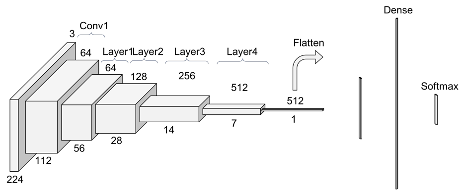 ","execution_count":null},{"metadata":{"trusted":true},"cell_type":"code","source":"class ResNet34Network(nn.Module):\n def __init__(self, output_size):\n super().__init__()\n \n # Define Feature part\n self.features = resnet34(pretrained=True)\n \n # Define Classification part\n self.classification = nn.Linear(1000, output_size)\n \n \n def forward(self, image, prints=False):\n if prints: print('Input Image shape:', image.shape)\n \n image = self.features(image)\n if prints: print('Features Image shape:', image.shape)\n \n out = self.classification(image)\n if prints: print('Out shape:', out.shape)\n \n return out","execution_count":null,"outputs":[]},{"metadata":{},"cell_type":"markdown","source":"### How is the Model working?\n
 ","execution_count":null},{"metadata":{"trusted":true,"_kg_hide-output":true},"cell_type":"code","source":"# Create an example model\nmodel_example = ResNet34Network(output_size=num_classes)","execution_count":null,"outputs":[]},{"metadata":{"trusted":true},"cell_type":"code","source":"# Data object and Loader\nexample_data = AlaskaDataset(train_df, is_test=False, is_val=False)\nexample_loader = torch.utils.data.DataLoader(example_data, batch_size = 1, shuffle=True)\n\n# Get a sample\nfor image, labels in example_loader:\n images_example = image\n labels_example = torch.tensor(labels, dtype=torch.long)\n break\nprint('Images shape:', images_example.shape)\nprint('Labels:', labels, '\\n')\n\n# Outputs\nout = model_example(images_example, prints=True)\n\n# Criterion example\ncriterion_example = nn.CrossEntropyLoss()\nloss = criterion_example(out, labels_example)\nprint('Loss:', loss.item())","execution_count":null,"outputs":[]},{"metadata":{},"cell_type":"markdown","source":"# 4. Data Prep 💽","execution_count":null},{"metadata":{"trusted":true},"cell_type":"code","source":"# ----- STATICS -----\nvertical_flip = 0.5\nhorizontal_flip = 0.5\n# -------------------","execution_count":null,"outputs":[]},{"metadata":{"trusted":true},"cell_type":"code","source":"# Data Objects\ntrain_data = AlaskaDataset(train_df, is_test=False, is_val=False, \n vertical_flip=vertical_flip, horizontal_flip=horizontal_flip)\nvalid_data = AlaskaDataset(valid_df, is_test=False, is_val=True, \n vertical_flip=vertical_flip, horizontal_flip=horizontal_flip)","execution_count":null,"outputs":[]},{"metadata":{},"cell_type":"markdown","source":"# 5. Train and Weighted AUC Functions 💾\n\n> Note: Function from notebook [Weighted AUC Metric (Updated)](https://www.kaggle.com/anokas/weighted-auc-metric-updated)\n\n* Optimizer:\n * The original `Adam` algorithm was proposed in `Adam: A Method for Stochastic Optimization`\n * The `AdamW` variant was proposed in `Decoupled Weight Decay Regularization`\n \n
Note to self: Try different Criterions and Optimizers.
\n ","execution_count":null},{"metadata":{"trusted":true},"cell_type":"code","source":"def train(model, epochs, batch_size, num_workers, learning_rate, weight_decay, \n version = 'vx', plot_loss=False):\n # Create file to save logs\n f = open(f\"logs_{version}.txt\", \"w+\")\n \n # Best AUC value\n best_auc = None \n \n # Data Loaders\n train_loader = torch.utils.data.DataLoader(train_data, batch_size=batch_size, num_workers=num_workers,\n drop_last=True, shuffle=True)\n valid_loader = torch.utils.data.DataLoader(valid_data, batch_size=batch_size, num_workers=num_workers,\n drop_last=True, shuffle=True)\n\n # Criterion\n criterion = torch.nn.CrossEntropyLoss()\n # Optimizer\n optimizer = optim.AdamW(model.parameters(), lr=learning_rate, weight_decay=weight_decay)\n # Scheduler\n scheduler = torch.optim.lr_scheduler.ReduceLROnPlateau(optimizer=optimizer, mode='max',\n patience=1, verbose=True, factor=0.4)\n\n\n train_losses = []\n evaluation_losses = []\n\n for epoch in range(epochs):\n\n # Sets the model in training mode\n model.train()\n\n train_loss = 0\n\n for images, labels in train_loader:\n # Need to access the images\n images = images.to(device, dtype=torch.float)\n labels = labels.to(device, dtype=torch.long)\n\n # Clear gradients\n optimizer.zero_grad()\n\n # Make prediction\n out = model(images)\n\n # Compute loss and Backpropagate\n loss = criterion(out, labels)\n loss.backward()\n optimizer.step()\n\n train_loss += loss.item()\n\n # Compute average epoch loss\n epoch_loss_train = train_loss / batch_size\n train_losses.append(epoch_loss_train)\n\n\n # ===== Evaluate =====\n model.eval()\n\n evaluation_loss = 0\n actuals, predictions = [], []\n\n # To disable gradients\n with torch.no_grad():\n for images, labels in valid_loader:\n images = images.to(device, dtype=torch.float)\n labels = labels.to(device, dtype=torch.long)\n\n # Prediction\n out = model(images)\n loss = criterion(out, labels)\n actuals.extend(labels.cpu().numpy().astype(int))\n predictions.extend(F.softmax(out, 1).cpu().numpy())\n\n evaluation_loss += loss.item()\n\n # Compute epoch loss\n epoch_loss_eval = evaluation_loss/batch_size\n evaluation_losses.append(epoch_loss_eval)\n\n # Prepare predictions and actuals\n predictions = np.array(predictions)\n # Choose label (array)\n predicted_labels = predictions.argmax(1)\n\n # ----- Accuracy -----\n accuracy = (predicted_labels == actuals).mean()\n\n # Compute AUC\n new_preds = np.zeros(len(predictions))\n temp = predictions[predicted_labels != 0, 1:]\n\n new_preds[predicted_labels != 0] = temp.sum(1)\n new_preds[predicted_labels == 0] = 1 - predictions[predicted_labels == 0, 0]\n actuals = np.array(actuals)\n actuals[actuals != 0] = 1\n\n auc_score = alaska_weighted_auc(actuals, new_preds)\n\n\n with open(f\"logs_{version}.txt\", 'a+') as f:\n print('Epoch: {}/{} | Train Loss: {:.3f} | Eval Loss: {:.3f} | AUC: {:3f} | Acc: {:3f}'.\\\n format(epoch+1, epochs, epoch_loss_train, epoch_loss_eval, auc_score, accuracy), file=f)\n \n print('Epoch: {}/{} | Train Loss: {:.3f} | Eval Loss: {:.3f} | AUC: {:3f} | Acc: {:3f}'.\\\n format(epoch+1, epochs, epoch_loss_train, epoch_loss_eval, auc_score, accuracy))\n\n # Update AUC\n # If AUC is improving, then we also save model\n if best_auc == None:\n best_auc = auc_score\n torch.save(model.state_dict(),\n f\"Epoch_{epoch+1}_ValLoss_{epoch_loss_eval:.3f}_AUC_{auc_score:.3f}.pth\")\n continue\n \n if auc_score > best_auc:\n best_auc = auc_score\n torch.save(model.state_dict(),\n f\"Epoch_{epoch+1}_ValLoss_{epoch_loss_eval:.3f}_AUC_{auc_score:.3f}.pth\")\n \n # Update scheduler (for learning_rate)\n scheduler.step(auc_score)\n \n # Plots the loss of Train and Valid\n if plot_loss:\n plt.figure(figsize=(14,5))\n plt.plot(train_losses, c='#fdc975ff', lw = 3)\n plt.plot(evaluation_losses, c='#29896bff', lw = 3)\n plt.legend(['Train Loss', 'Evaluation Loss'])\n plt.title('Losses over Epochs');","execution_count":null,"outputs":[]},{"metadata":{},"cell_type":"markdown","source":"# 6. Training...💻✔","execution_count":null},{"metadata":{"trusted":true},"cell_type":"code","source":"# ----- STATICS -----\nversion = 'v8'\nepochs = 3\nbatch_size = 32\nnum_workers = 8\nlearning_rate = 0.001\nweight_decay = 0.00001\nplot_loss = False\n# -------------------","execution_count":null,"outputs":[]},{"metadata":{"trusted":true},"cell_type":"code","source":"# # Efficient Net B0\n# eff_net0 = EfficientNetwork(output_size = num_classes, b1=False, b2=False).to(device)\n\n# # Load any pretrained model\n# eff_net0.load_state_dict(torch.load('../input/v2-effnet-epoch-6-auc-08023/10Class_epoch_14_val_loss_77.34_auc_0.78_EffNetB0.pth'))\n\n# # Uncomment and train the model\n# train(model=eff_net0, epochs=epochs, batch_size=batch_size, num_workers=num_workers, \n# learning_rate=learning_rate, weight_decay=weight_decay, plot_loss=plot_loss)","execution_count":null,"outputs":[]},{"metadata":{"trusted":true},"cell_type":"code","source":"# Efficient Net B2\neff_net2 = EfficientNetwork(output_size = num_classes, b1=False, b2=True).to(device)\n\n# # Add previous trained model:\n# eff_net2.load_state_dict(torch.load('../input/v2-effnet-epoch-6-auc-08023/Epoch_7_ValLoss_58.146_AUC_0.799.pth'))\n\n# Uncomment and train the model\n# train(model=eff_net2, epochs=epochs, batch_size=batch_size, num_workers=num_workers, \n# learning_rate=learning_rate, weight_decay=weight_decay, plot_loss=plot_loss)","execution_count":null,"outputs":[]},{"metadata":{"trusted":true,"_kg_hide-output":false},"cell_type":"code","source":"# # ResNet34\n# eff_net34 = ResNet34Network(output_size = num_classes).to(device)\n\n# # Uncomment and train the model\n# train(model=eff_net34, epochs=epochs, batch_size=batch_size, num_workers=num_workers, \n# learning_rate=learning_rate, weight_decay=weight_decay, plot_loss=plot_loss)","execution_count":null,"outputs":[]},{"metadata":{},"cell_type":"markdown","source":"# 7. Inference 📈\n\n## 7.1 Data","execution_count":null},{"metadata":{"trusted":true},"cell_type":"code","source":"# Extract a sample of paths\ndirectory = '../input/alaska2-image-steganalysis/'\nname = pd.Series(sorted(os.listdir(directory + 'Test/')))\npath = pd.Series(directory + 'Test/' + name)\n\n# Create dataframe\ntest_df = pd.DataFrame(data=path, columns=['Path'])\n\n# Dataset\ntest_data = AlaskaDataset(test_df, is_test=True, is_val=False,\n vertical_flip=vertical_flip, horizontal_flip=horizontal_flip)\ntest_loader = torch.utils.data.DataLoader(test_data, batch_size = batch_size, shuffle=False)","execution_count":null,"outputs":[]},{"metadata":{},"cell_type":"markdown","source":"## 7.2 Predict","execution_count":null},{"metadata":{"trusted":true},"cell_type":"code","source":"# list(os.listdir('../working/Epoch_17_ValLoss_36.195_AUC_0.794.pth'))\n\n# Import model if necessary:\n# Load any pretrained model\n# eff_net2.load_state_dict(torch.load('../working/Epoch_17_ValLoss_36.195_AUC_0.794.pth'))","execution_count":null,"outputs":[]},{"metadata":{"trusted":true},"cell_type":"code","source":"# Evaluation Mode\neff_net2.eval()\n\npredictions = []\n\nwith torch.no_grad():\n for k, images in enumerate(test_loader):\n images = images.to(device)\n out0 = eff_net2(images)\n \n # Flip vertical\n images_vertical = images.flip(2)\n out1 = eff_net2(images_vertical)\n \n # Flip again original\n images_flip = images.flip(3)\n out2 = eff_net2(images_flip)\n \n # 50% results from flip + 50% result from normal\n outputs = (0.25*out1 + 0.25*out2)\n outputs = (outputs + 0.5*out0)\n\n predictions.extend(F.softmax(outputs, 1).cpu().numpy())","execution_count":null,"outputs":[]},{"metadata":{"trusted":true},"cell_type":"code","source":"# Making the predictions the same manner as in Train Function\npredictions = np.array(predictions)\npredicted_labels = predictions.argmax(1)\nnew_preds = np.zeros(len(predictions))\ntemp = predictions[predicted_labels != 0, 1:]\nnew_preds[predicted_labels != 0] = temp.sum(1)\nnew_preds[predicted_labels == 0] = 1 - predictions[predicted_labels == 0, 0]","execution_count":null,"outputs":[]},{"metadata":{},"cell_type":"markdown","source":"### Submission File\n\n> Note: The submission will actually deliver only if you train on more datapoints (this is just a very small sample so the notebook runs fast :) )","execution_count":null},{"metadata":{"trusted":true},"cell_type":"code","source":"ss = pd.read_csv('../input/alaska2-image-steganalysis/sample_submission.csv')\nss['Label'] = new_preds\n\nss.to_csv(f'submission_{version}.csv', index=False)","execution_count":null,"outputs":[]},{"metadata":{},"cell_type":"markdown","source":"
EffNet B0 (10 class): 30,000 sample_size | 19 epochs | 16 batch_size | LB Score is 0.822.
\nEffNet B2 (10 class): 70,000 sample_size | 15 epochs | 16 batch_size | LB Score is 0.805.
\nWorking to make it better.
\nIf you liked this, upvote!
\nCheers!
\n