{"cells":[{"metadata":{"_uuid":"e54e6153602d2b41872662fb0cc78c6b44854ed2"},"cell_type":"markdown","source":"This notebook is a very quick overview of the dataset for the PLAsTiCC Astronomical Classification competition, and intends to be a first exploration notebook to get used to the dataset.\n\n# Table of contents\n___\n- [Data overview and target identification](#overview)\n- [DDF areas](#ddfs)\n- [Distmod and redshift](#distred)\n- [Galactical versus Extragalactical sources](#galvsextra)\n- [Passband](#passband)\n- [Flux time plots](#fluxplots)"},{"metadata":{"_uuid":"8f2839f25d086af736a60e9eeb907d3b93b6e0e5","_cell_guid":"b1076dfc-b9ad-4769-8c92-a6c4dae69d19","trusted":true},"cell_type":"code","source":"import numpy as np # linear algebra\nimport pandas as pd # data processing, CSV file I/O (e.g. pd.read_csv)\nimport seaborn as sb\nimport matplotlib.pyplot as plt\n%matplotlib inline\n#read csv\ntraining = pd.read_csv('../input/training_set.csv')","execution_count":null,"outputs":[]},{"metadata":{"_uuid":"d4b5eebbdc2f50f902c0f48d663bdc6815c24d4d"},"cell_type":"markdown","source":"# Data overview and target identification \n___\nFirst of all, let's take a look at the dataset. "},{"metadata":{"_cell_guid":"79c7e3d0-c299-4dcb-8224-4455121ee9b0","_uuid":"d629ff2d2480ee46fbb7e2d37f6b5fab8052498a","trusted":true,"scrolled":true},"cell_type":"code","source":"training.sample(5)","execution_count":null,"outputs":[]},{"metadata":{"_uuid":"e0c67b4a4f67df6e08a143601469e63ef1f70a4b"},"cell_type":"markdown","source":"So there are 6 fields in total. These are:\n- mjd: the time in Modified Julian Date (MJD) of the observation. Can be read as days since November 17, 1858. Can be converted to Unix epoch time with the formula unix_time = (MJD−40587)×86400. \n- passband: The specific LSST passband integer, such that u, g, r, i, z, Y = 0, 1, 2, 3, 4, 5 in which it was viewed. \n- flux: the measured flux (brightness) in the passband of observation as listed in the passband column. These values have already been corrected for dust extinction (mwebv), though heavily extincted objects will have larger uncertainties (flux_err) in spite of the correction. \n- flux_err: the uncertainty on the measurement of the flux listed above. \n- detected: If 1, the object's brightness is significantly different at the 3-sigma level relative to the reference template. Only objects with at least 2 detections are included in the dataset. \n\nBesides those columns, we have another dataset, `training_set_metadata.csv`, in which we can find the following fields:"},{"metadata":{"trusted":true,"scrolled":true,"_uuid":"338cfeb64bcab0ee020a8f1599f141efcf6c45f9"},"cell_type":"code","source":"meta_training = pd.read_csv(\"../input/training_set_metadata.csv\")\nmeta_training.sample(5)","execution_count":null,"outputs":[]},{"metadata":{"_uuid":"361cdcf651216ea2cb5a6f6042d231cd1a480cdb"},"cell_type":"markdown","source":"Where each column represents:\n\n- object_id: unique object identifier.\n- ra: right ascension, sky coordinate: co-longitude in degrees. \n- decl: declination, sky coordinate: co-latitude in degrees. \n- gal_l: galactic longitude in degrees. \n- gal_b: galactic latitude in degrees. \n- ddf: A flag to identify the object as coming from the DDF survey area (with value DDF = 1 for the DDF, DDF = 0 for the WFD survey). Note that while the DDF fields are contained within the full WFD survey area, the DDF fluxes have significantly smaller uncertainties. Boolean\n- hostgal_specz: the spectroscopic redshift of the source. This is an extremely accurate measure of redshift, available for the training set and a small fraction of the test set. \n- hostgal_photoz: The photometric redshift of the host galaxy of the astronomical source. While this is meant to be a proxy for hostgal_specz, there can be large differences between the two and should be regarded as a far less accurate version of hostgal_specz. \n- hostgal_photoz_err: The uncertainty on the hostgal_photoz based on LSST survey projections. \n- distmod: The distance to the source calculated from hostgal_photoz and using general relativity.\n- mwebv: MW E(B-V). this ‘extinction’ of light is a property of the Milky Way (MW) dust along the line of sight to the astronomical source, and is thus a function of the sky coordinates of the source ra, decl. This is used to determine a passband dependent dimming and redenning of light from astronomical sources as described in subsection 2.1, and based on the Schlafly et al. (2011) and Schlegel et al. (1998) dust models. \n- target: The class of the astronomical source. This is provided in the training data. Correctly determining the target (correctly assigning classification probabilities to the objects) is the ‘goal’ of the classification challenge for the test data. Note that there is one class in the test set that does not occur in the training set: class_99 serves as an \"other\" class for objects that don't belong in any of the 14 classes in the training set. \n\nLet's explore a bit the target variable first. "},{"metadata":{"trusted":true,"_uuid":"b89f212c6cb8d8636f0d8957e8545a43287e2c64"},"cell_type":"code","source":"unique_targets = meta_training.target.unique()\nprint (\"There are {} unique targets.\".format(len(unique_targets)))\nprint (unique_targets)","execution_count":null,"outputs":[]},{"metadata":{"_uuid":"216d7aeb2d9e2315a97d7b9f00df7eb7c7e8ad82"},"cell_type":"markdown","source":"Our goal, then is to classify our objects into one of those 14 classes. Just as a reminder, there is one more class, 99, that is present in the test set but not in the dataset. As the description from the challenge mentions, this serves as a placeholder for objects that don't belong to any of the 14 classes in the training set."},{"metadata":{"trusted":true,"_uuid":"cebf74fdf5a08e9a751bc880a055efbeaaafaf16"},"cell_type":"code","source":"objects_per_target = pd.DataFrame(meta_training.groupby(\"target\", as_index = False)[\"object_id\"].count())\nobjects_per_target = objects_per_target.rename(columns = {\"object_id\": \"num_of_objects\"})\nfig = plt.figure(figsize=(10,8))\nsb.barplot(x =objects_per_target.target, y = objects_per_target.num_of_objects);","execution_count":null,"outputs":[]},{"metadata":{"_uuid":"9c87737945819594f6557e56a8a587bd2950e872"},"cell_type":"markdown","source":"Most objects are from class 90, followed by classes 42, 16 and 15, while just a few are from class 53. \n\nNow we'll get some intuition on how those classes are spread in space."},{"metadata":{"trusted":true,"_uuid":"788a4325ff5935d3e2d77e8940b6dca29b7caafc"},"cell_type":"code","source":"fig = plt.figure(figsize=(10,8))\nax = fig.add_subplot(111)\nfor class_target in unique_targets:\n class_used = meta_training[meta_training.target == class_target]\n ax.scatter(x = class_used.gal_l, y = class_used.gal_b, alpha = 1)\nplt.xlabel(\"Galactical Longitude(°)\", fontsize = 15)\nplt.ylabel(\"Galactical Latitude(°)\", fontsize = 15);","execution_count":null,"outputs":[]},{"metadata":{"_uuid":"e3f056c541193e070feb643ba37d2a924be4573a"},"cell_type":"markdown","source":"Apparently, there is nothing very specific in this graph. All kinds of galaxies can be found in pretty much everywhere in the sky. Its strange form is probably due to where the detectors are placed and their sky coverage. \nBy reading the map below, I think the map can see most of the Americas' sky (considering the increase in angle going from left to right.\n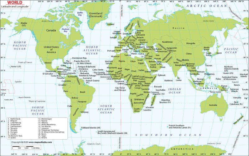\n\nHowever, it might be useful to lower alpha parameter to see if we can find spots that have a higher density of objects."},{"metadata":{"trusted":true,"_uuid":"faf49c0821a421c9a322285a627b0fc9420df90e"},"cell_type":"code","source":"fig = plt.figure(figsize=(10,8))\nax = fig.add_subplot(111)\nfor class_target in unique_targets:\n class_used = meta_training[meta_training.target == class_target]\n ax.scatter(class_used.gal_l,class_used.gal_b, alpha = .1)\nax.set_xlabel(\"Galactical Longitude (°)\", fontsize = 15)\nax.set_ylabel(\"Galactical Latitude (°)\", fontsize = 15);","execution_count":null,"outputs":[]},{"metadata":{"_uuid":"f0d810b491d63ced3cc7ecbaf861129947431195"},"cell_type":"markdown","source":"# DDF areas \n___\nNow we found something peculiar. There are five spots in the sky with a high density of observed objects. These particular spots may point out to nice insights if worked on properly. The points seem to be around these intervals:\n- [-60º:-57º, 165º:180º]\n- [-56º:-53º, 220º:225º]\n- [40º:43º, 228º:235º]\n- [-53º:-51º, 315º:323º]\n- [-72º:-75º, 322º, 332º]\n\nOne things that is worthy pointing out is that four of those five clusters of objects are below 40º South, one of them even below the Antartic circle. I'm not sure this will be relevant at some point, but insights are insights, right? \nNow, it is worth looking at those intervals to see if we can find some kind of pattern. "},{"metadata":{"trusted":true,"_uuid":"a7a4f7e2f2de504e98651bcb09c5e485e0828445"},"cell_type":"code","source":"condition = (round(meta_training[\"gal_b\"]).isin(range(38,48)) & round(meta_training[\"gal_l\"]).isin(range(226,238)))\\\n |(round(meta_training[\"gal_b\"]).isin(range(-56,-52)) & round(meta_training[\"gal_l\"]).isin(range(220,226)))\\\n |(round(meta_training[\"gal_b\"]).isin(range(-66,-56)) & round(meta_training[\"gal_l\"]).isin(range(165,178)))\\\n |(round(meta_training[\"gal_b\"]).isin(range(-55,-45)) & round(meta_training[\"gal_l\"]).isin(range(315,323)))\\\n |(round(meta_training[\"gal_b\"]).isin(range(-77,-65)) & round(meta_training[\"gal_l\"]).isin(range(322,332)))\nfive_point = meta_training.loc[condition]\n\nfig = plt.figure(figsize=(10,8))\nax = fig.add_subplot(111)\nfor class_target in unique_targets:\n class_used = five_point[five_point.target == class_target]\n ax.scatter(class_used.gal_l,class_used.gal_b, alpha = .1)\nax.set_xlabel(\"Galactical Longitude (°)\", fontsize = 15)\nax.set_ylabel(\"Galactical Latitude (°)\", fontsize = 15);","execution_count":null,"outputs":[]},{"metadata":{"_uuid":"0763baf22fa27661dd05d61e1bcb1bb689951f64"},"cell_type":"markdown","source":"Great! Now we got our points. I didn't use the exact intervals I proposed before due to trial and error. Some of them were too small and I had to tweak a bit in order to get the whole cluster. Now let's check the class distribution to see if it's somehow different."},{"metadata":{"trusted":true,"_uuid":"bf0a05ca5b1f757838834dbd5f3f42c48ee72bf6"},"cell_type":"code","source":"objects_per_target_five = pd.DataFrame(five_point.groupby(\"target\", as_index = False)[\"object_id\"].count())\nobjects_per_target_five = objects_per_target_five.rename(columns = {\"object_id\": \"num_of_objects\"})\nfig = plt.figure(figsize=(10,8))\nsb.barplot(x =objects_per_target_five.target, y = objects_per_target_five.num_of_objects);\nplt.xlabel(\"Class\", fontsize = 15)\nplt.ylabel(\"Number of sources\", fontsize = 15);","execution_count":null,"outputs":[]},{"metadata":{"_uuid":"022d95d96524a2d64c2500bd3facd62a3ed0c7dd"},"cell_type":"markdown","source":"Seems to me that nothing has changed much. There are proportionally fewer class 15 objects but I'm not sure if this is just some random fluctuation or an important feature. I tend to think it is the former, but anyway, just exploring the possibilities :) Further tests are needed to confirm or reject this hypothesis. \n\nOne thing that just caught my attention while exploring, looking for possible features where patterns could be found, is the `ddf` column. If 1, it means the object was observed from within a specific area (DDF survey area). So, maybe... Yeah, let's try that! First, the counts of ddf objects in the original meta_training dataset."},{"metadata":{"trusted":true,"_uuid":"bedf9e525477d6c3ebaec76764cdc4b794b18930"},"cell_type":"code","source":"ddf_counts = pd.DataFrame(meta_training.groupby(\"ddf\", as_index = False)[\"object_id\"].count())\nddf_counts","execution_count":null,"outputs":[]},{"metadata":{"_uuid":"631d4642a9e9139b34b42f98fdcedaf91e8a45a0"},"cell_type":"markdown","source":"So the proportion is about 2 ddf objects to each 5 objects detected. Now, the clusters..."},{"metadata":{"trusted":true,"_uuid":"928b879f08785a6a0053727d3b429988a341144d"},"cell_type":"code","source":"ddf_counts_five = pd.DataFrame(five_point.groupby(\"ddf\", as_index = False)[\"object_id\"].count())\nddf_counts_five","execution_count":null,"outputs":[]},{"metadata":{"_uuid":"44d3f6a4ce458cfcceca699d64e649f5cb7ea3ac"},"cell_type":"markdown","source":"Woah! I guess the DDF survey areas were found :P Each of the five clusters is such distinct area. The 26 objects are there probably due to my latitude/longitude choice, and that's the same reason the other 107 ddf objects aren't there as well. Maybe there are other features that could be seen only in those regions? The only thing we have for granted, according to the information provided by the organizers, is that DDF fluxes have smaller uncertainties compared to the others. In my opinion, these won't turn out to be really special places except for the fact that these are the places where the DDFs were built. In [slide 13](https://project.lsst.org/groups/sac/sites/lsst.org.groups.sac/files/Brandt_DDF.pdf) is possible to see where they are located. I couldn't find one of them on that image, though. \n\nWhile we are at the galactical coordinates of the objects, we can check if the distances vary with galaxy coordinates - i.e. we want to check if we looked to right, distances from the objects would be, on average, the same as if we looked to other direction."},{"metadata":{"trusted":true,"_uuid":"4831c6d5d3901d0fca399d9f4705432485d3fc21"},"cell_type":"code","source":"fig = plt.figure(figsize=(10,8))\nax = fig.add_subplot(111)\nax.scatter(meta_training.gal_l,meta_training.gal_b, c = meta_training.distmod, s = 7, cmap = 'Reds');\nax.set_xlabel(\"Galactical Longitude (°)\", fontsize = 15)\nax.set_ylabel(\"Galactical Latitude (°)\", fontsize = 15);","execution_count":null,"outputs":[]},{"metadata":{"_uuid":"059949ed3b34efe628978b11ad3cda0dc57f3321"},"cell_type":"markdown","source":"The distances seem to be pretty random - which seems to agree with the isotropy of the universe (it looks the same in all directions). But although they are the same in about every direction, perhaps there is a difference between close and far source counts. Are there more sources closer or distant from us?\n\n# Distmod and redshift \n___"},{"metadata":{"trusted":true,"_uuid":"9a506ac7d00eaa2ff0a8fc2a0e19af039cf016ec"},"cell_type":"code","source":"fig = plt.figure(figsize=(10,8))\nsb.distplot(meta_training[~np.isnan(meta_training.distmod)].distmod);\n# plt.xlabel(\"Distance to the source\")\nplt.ylabel(\"Frequency\", fontsize = 15);\nplt.xlabel(\"Distmod\", fontsize = 15);","execution_count":null,"outputs":[]},{"metadata":{"_uuid":"a640fb6970e7848f46d8acfba2a4a9e57a4fa730"},"cell_type":"markdown","source":"So the distribution of source distances is (close to) binormal, with peaks around 41 and 47. Now, is there any relationship between the redshift observed and the distance they are?"},{"metadata":{"trusted":true,"scrolled":true,"_uuid":"6ce7f0e4b015f63e041aebd5ff1c72345fd72e6f"},"cell_type":"code","source":"meta_training.distmod.corr(meta_training.hostgal_photoz)","execution_count":null,"outputs":[]},{"metadata":{"_uuid":"fd78a045f67870f81f7a82d326d75c9a6fc49146"},"cell_type":"markdown","source":"Well, that's a fairly high correlation. Let's plot to visually confirm what's going on here:"},{"metadata":{"trusted":true,"_uuid":"983eafc418416a7259ce7f62abc042154d78bab0"},"cell_type":"code","source":"fig = plt.figure(figsize=(10,8))\nplt.scatter(meta_training.distmod, meta_training.hostgal_photoz, s = 1);\nplt.xlabel(\"Distmod\", fontsize = 15);\nplt.ylabel(\"Host Galaxy Photometric Redshift\", fontsize = 15);","execution_count":null,"outputs":[]},{"metadata":{"_uuid":"1e08051a61b14524d6ddcec06783f9c2eaf4b2f0"},"cell_type":"markdown","source":"\nYeah, there is definitely something non-trivial going on here. The farther a source (and thus their host galaxy) is, more is the [redshift](https://en.wikipedia.org/wiki/Redshift). this indicates that the farther the sources (and host galaxies) are, the faster they are moving away from us. I decided to go with the photoz variable rather than specz because this is not available for most of the test site and although far less accurate according to the data description, it seems to be more useful. Moreover, we should also see how the error in hostgal_photoz behaves."},{"metadata":{"trusted":true,"scrolled":true,"_uuid":"7f61a8301e5bb75c0d6f31890b5de94b1d6aad97"},"cell_type":"code","source":"fig = plt.figure(figsize=(10,8))\nplt.scatter(meta_training.distmod, meta_training.hostgal_photoz_err, s = 1);\nplt.xlabel(\"Distmod\", fontsize = 15);\nplt.ylabel(\"Host Galaxy Photometric Redshift Error\", fontsize = 15);","execution_count":null,"outputs":[]},{"metadata":{"_uuid":"2fe35e9c583f6746c604c3f3cb3183a8943f1c8d"},"cell_type":"markdown","source":"Seems like most errors are small, but there certainly are some big errors as high as the same order of magnitude of the measures themselves. Although not perfect, that's what we got to work with.\n\nJust to be sure, we can also plot specz as a function of the distance to the source."},{"metadata":{"trusted":true,"_uuid":"1823929e91ffa1f5643f75f65cd867267d458c6b"},"cell_type":"code","source":"fig = plt.figure(figsize=(10,8))\nplt.scatter(meta_training.distmod, meta_training.hostgal_specz, s = 1);\nplt.xlabel(\"Distmod\", fontsize = 15);\nplt.ylabel(\"Host Galaxy Spectroscopic Redshift\", fontsize = 15);","execution_count":null,"outputs":[]},{"metadata":{"_uuid":"a529e8dd8a82c5e9683dd7dbf53a42c7005b2d8a"},"cell_type":"markdown","source":"Indeed, although there is some resemblance to photoz, there are lot of points spread out and also a cluster on the bottom edge of the scatterplot showing objects with a very low redshift, meaning that although their host galaxies are moving fast away from us, the sources themselves are moving slower. \n\n# Galactical versus Extragalactical Sources \n___\nIt is mentioned in the [starter kit](https://www.kaggle.com/michaelapers/the-plasticc-astronomy-starter-kit) and also used in [Kyle's notebook](https://www.kaggle.com/kyleboone/naive-benchmark-galactic-vs-extragalactic) the fact that galactic and extragalactic sources are easily separated, and the organizers simulated this feature by setting redshift from galactic sources to exactly `0`. I think it is worthy checking if these two source types have differences regarding the other aspects we've seen so far."},{"metadata":{"trusted":true,"_uuid":"9e692f84eb6e062e67ec99969056a2e17d0ae272"},"cell_type":"code","source":"#first we should split the dataset between galactic and extragalactic sources\ngalactic = meta_training[meta_training.hostgal_photoz == 0]\ngalactic.sample(5)","execution_count":null,"outputs":[]},{"metadata":{"_uuid":"c433a1151e61dfdb2662c470d9b3d10c94856999"},"cell_type":"markdown","source":"Two key points that call the attention here:\n- Even though photoz is just a proxy to photoz, they are both zero for galactic sources;\n- distmod is `NaN` to all of them.\n\nNow, let's define and check the extragalactic subset"},{"metadata":{"trusted":true,"scrolled":true,"_uuid":"49bf2f68d5e7beec93c3d822b830d011c6bde254"},"cell_type":"code","source":"extragalactic = meta_training[meta_training.hostgal_photoz != 0]\nextragalactic.sample(5)","execution_count":null,"outputs":[]},{"metadata":{"_uuid":"f455b374e3bd430b47c7e1521107f518a717733b"},"cell_type":"markdown","source":"It is also possible to check that there are no null values for extragalactic `distmod`. Hence all the nulls presented in this variable are not due to errors in simulation nor at random, and this can be confirmed in the starter's kit as well, a few paragraphs below figure 27., when the authors say \"For galactic objects with `hostgal_photoz = 0` , the distmod is reported as `NaN` (the distance would be 0, and taking the logarithm of 0 is a bad idea).\" I missed that part when I read their notebook at first (it's a loooong notebook :P) and only checked the information after finding this here, so I decided to keep this analysis for people who might miss this information just like I did. \n\nWe've just got our galactic and extragalactic datasets, so let's check their differences!"},{"metadata":{"trusted":true,"_uuid":"f177d955cd7dd3bdef686fc434175a1c37754a76","scrolled":true},"cell_type":"code","source":"#for convinience while making the plots, I'll create a variable to reference the galactic/extragalactic feature. 1 for extragalactic and 0 for galactic\nmeta_training['extra'] = 0\nmeta_training.loc[meta_training.hostgal_photoz != 0, 'extra'] = 1\n\n# plt.hist(meta_training[meta_training.extra == 0].target, label = 'Galactic')\n\nmeta_training['target'] = meta_training['target'].astype('category',copy=False)\n\ngrid = sb.FacetGrid(data = meta_training, hue = 'extra', height =7)\ngrid.map(sb.countplot, 'target')\nfor ax in grid.axes.ravel():\n ax.legend()\nplt.xlabel(\"Class\", fontsize = 15)\nplt.ylabel(\"Counts\", fontsize = 15);","execution_count":null,"outputs":[]},{"metadata":{"_uuid":"8bf6f4964d87408b2e013847e8ad2c8330166d30"},"cell_type":"markdown","source":"Excellent! When we are only dealing with galactic sources, we'll effectively be labeling five classes, and 9 classes when dealing with extragalactic sources. Note that class overlaps between different source types do not occur."},{"metadata":{"trusted":true,"_uuid":"ceefe7d3e14a9d550d9873cee5ead449c1330961"},"cell_type":"code","source":"fig = plt.figure(figsize=(10,8))\nplt.scatter(x = galactic.gal_l, y = galactic.gal_b, alpha = 0.5, label = 'galactic')\nplt.scatter(x = extragalactic.gal_l, y = extragalactic.gal_b, alpha = 0.1, label = 'extragalactic');\nplt.xlabel(\"Galactic longitude (°)\", fontsize = 15)\nplt.ylabel(\"Galactic latitude (º)\", fontsize = 15)\nplt.legend();","execution_count":null,"outputs":[]},{"metadata":{"_uuid":"cca02365fd4e9ec44e30c9a6889a231d31ee5cbe"},"cell_type":"markdown","source":"I set different alpha parameters so we can confirm superpose both set of points and visualize the result. As expected, both types of objects can be seen in all directions (isotropic universe). Although it does not look like so in this plot, DDF regions are also capable of detecting several galactic points and the only reason extragalactic points are standing out in this plot is because the orange points are being ploted right above the blue ones. If the scatterplots are done in different subplots, it is possible to see both blue and orange points there. \n\nNow that we've talked about the meta training data, let's see the behaviour of the training data. Before going further on this analysis, I think it will be helpful to merge both datasets so we can see some of the training fields from the perspective of a few meta training fields in case we want to. "},{"metadata":{"trusted":true,"scrolled":false,"_uuid":"9fbca028e9371a951ed0e91cf3d199c319a7ac79"},"cell_type":"code","source":"merged = training.merge(meta_training, on = \"object_id\")\nmerged.sample(5)","execution_count":null,"outputs":[]},{"metadata":{"_uuid":"49b2ec86f64d495b79ed458d95c942397e506ba3"},"cell_type":"markdown","source":"# Passband \n___ \nBefore going into the flux plots, which are think are one of the most interesting and important parts of the dataset, I'd like to make a short analysis on the passband filters, since they will be seen in flux time plots as well.\n\nFirst, let's see the use of passband filters. Is anyone of them used more often than the others?"},{"metadata":{"trusted":true,"_uuid":"b3cd05974b0a15c7dfc3d2edd0b6e75f311b0a9a"},"cell_type":"code","source":"grid = sb.FacetGrid(data = merged, height =7)\ngrid.map(sb.countplot, 'passband')\nfor ax in grid.axes.ravel():\n ax.legend()\nplt.xlabel(\"Passband\", fontsize = 15)\nplt.ylabel(\"Counts\", fontsize = 15);","execution_count":null,"outputs":[]},{"metadata":{"_uuid":"b3b35972e3b08ec40edcb6ff0aa981979d34464e"},"cell_type":"markdown","source":"Let's remember the filters used: {u→0, g→1, r→2, i→3, z→4, y→5} where \"u covers the ultraviolet, g covers what your eye perceives as blue/green, r covers red, i covers the infrared\". The z and y filters don't have any particular reason to be named that way, and further information on this can be found [here](http://articles.adsabs.harvard.edu/cgi-bin/nph-iarticle_query?2008JAVSO..36..110M&data_type=PDF_HIGH&whole_paper=YES&type=PRINTER&filetype=.pdf). \n\nRegarding the plot, we can see that filters z and y are actually the most used, while green/blue filter is the less used one. So in the following plots, we'll see these two filters being used more often."},{"metadata":{"_uuid":"2368a47a5b8f7758476c2e2bbfebc522332e4cce"},"cell_type":"markdown","source":"# Flux time plots \n___\nI'll use only one object_id to get a feel of the data."},{"metadata":{"trusted":true,"scrolled":true,"_uuid":"8f8ce68e2e8dbd5030deec1fdbd4b1aa7ce31446"},"cell_type":"code","source":"unique_sources = merged.object_id.unique()\nobj_data = merged[merged.object_id == unique_sources[0]]\nobj_data.head(5)","execution_count":null,"outputs":[]},{"metadata":{"_uuid":"b4db8c669b02f7f082e9bbebd15cde8cd1c6967b"},"cell_type":"markdown","source":"The chosen object (615) is a galactic source in the DDF area and belongs to class 92. Let's see how the flux in each passband varies with time (here measured in mjd). "},{"metadata":{"trusted":true,"scrolled":false,"_uuid":"e3286e4c8671c518e0b41e2f67125c37acce47cb"},"cell_type":"code","source":"unique_passbands = merged.passband.unique()\n\nfig = plt.figure(figsize=(10,8))\nfor passband in unique_passbands:\n specific_pb = obj_data[obj_data.passband == passband]\n plt.scatter(specific_pb.mjd, specific_pb.flux, label = passband)\nplt.xlabel(\"MJD (in days from November 17, 1858)\", fontsize = 15)\nplt.ylabel(\"Flux\", fontsize = 15)\nplt.legend();","execution_count":null,"outputs":[]},{"metadata":{"_uuid":"d510bd5f1332214b277e580b7269bb5231ad46b7"},"cell_type":"markdown","source":"This doesn't seem very helpful. We can see that there are three time windows from where the data is taken. Maybe we should focus on one of those windows to take a better understanding here. "},{"metadata":{"trusted":true,"scrolled":true,"_uuid":"3a3256de64ca816d0d0392c4e3413434add9193e"},"cell_type":"code","source":"window_objdata = obj_data[(obj_data.mjd > 60100) & (obj_data.mjd<60300)]\nfig = plt.figure(figsize=(15,8))\nfor passband in unique_passbands:\n specific_pb = window_objdata[window_objdata.passband == passband]\n plt.plot(specific_pb.mjd, specific_pb.flux, label = passband)\nplt.xlabel(\"MJD (in days from November 17, 1858)\", fontsize = 15)\nplt.ylabel(\"Flux\", fontsize = 15)\nplt.legend();","execution_count":null,"outputs":[]},{"metadata":{"_uuid":"829fb44b3f372b793f7eb382928b02eaaec88742"},"cell_type":"markdown","source":"The peaks here do seem to occur at the same time especially after the third one, but before that all seems to be messy. Starter kit's authors mentioned that different sources will show different behaviours in flux, so let's confirm that by looking at another class 92 object and after that two other similar objects from a different class."},{"metadata":{"trusted":true,"scrolled":false,"_uuid":"56fc953d019960e26997a0f49078e49a09121f5b"},"cell_type":"code","source":"#get objects from class 92\nclass_92_objs = merged[merged.target == 92]\n#unique objects from class 92\nunique_sources_92 = class_92_objs.object_id.unique()\n#get data from one specific object from class 92 (elemment 0 is the same from before)\nobj_data = merged[merged.object_id == unique_sources_92[4]]\n#get one time window to observe and plot\nwindow_objdata = obj_data[(obj_data.mjd > 60100) & (obj_data.mjd<60300)]\nfig = plt.figure(figsize=(15,8))\nfor passband in unique_passbands:\n specific_pb = window_objdata[window_objdata.passband == passband]\n plt.plot(specific_pb.mjd, specific_pb.flux, label = passband)\nplt.xlabel(\"MJD (in days from November 17, 1858)\", fontsize = 15)\nplt.ylabel(\"Flux\", fontsize = 15)\nplt.legend();","execution_count":null,"outputs":[]},{"metadata":{"_uuid":"12e0446d5918c0a9ac80778fd87ea0a2f59746d0"},"cell_type":"markdown","source":"Now let's do the same to another class, say 52."},{"metadata":{"trusted":true,"scrolled":false,"_uuid":"2102162f7be02a9d800c5eca68a510b5e414c245"},"cell_type":"code","source":"#get objects from class 52\nclass_52_objs = merged[merged.target == 52]\n#unique objects from class 52\nunique_sources_52 = class_52_objs.object_id.unique()\n#get data from one specific object from class 52\nobj_data = merged[merged.object_id == unique_sources_52[0]]\n#get one time window to observe and plot\nwindow_objdata = obj_data[(obj_data.mjd > 60100) & (obj_data.mjd<60300)]\nfig = plt.figure(figsize=(15,8))\nfor passband in unique_passbands:\n specific_pb = window_objdata[window_objdata.passband == passband]\n plt.plot(specific_pb.mjd, specific_pb.flux, label = passband)\nplt.xlabel(\"MJD (in days from November 17, 1858)\", fontsize = 15)\nplt.ylabel(\"Flux\", fontsize = 15)\nplt.legend();","execution_count":null,"outputs":[]},{"metadata":{"trusted":true,"scrolled":false,"_uuid":"ba2232f5607bdc528722ff233551a220378b27a6"},"cell_type":"code","source":"#get data from one specific object from class 52\nobj_data = merged[merged.object_id == unique_sources_52[2]]\n#get one time window to observe and plot\nwindow_objdata = obj_data[(obj_data.mjd > 60100) & (obj_data.mjd<60300)]\nfig = plt.figure(figsize=(15,8))\nfor passband in unique_passbands:\n specific_pb = window_objdata[window_objdata.passband == passband]\n plt.plot(specific_pb.mjd, specific_pb.flux, label = passband)\nplt.xlabel(\"MJD (in days from November 17, 1858)\", fontsize = 15)\nplt.ylabel(\"Flux\", fontsize = 15)\nplt.legend();","execution_count":null,"outputs":[]},{"metadata":{"_uuid":"ba9bf11082ce732c9fa41eacc25b7d2f2e51b37a"},"cell_type":"markdown","source":"So class 52 seems to have a very irregular flux pattern. I tested a few others from this class just to be sure, and the plots are very similar. Note that 52 is a class from an extragalactic source and 92 is from a galactic one. So maybe there is some kind of pattern? Perhaps galactic objects have a more regular structure that can be seen from a simple timeplot of its flux pattern while extragalactic objects are more irregular and to find out a characteristic time scale we would have to use more advanced methods, such as the suggested Lomb-Scargle Periodogram from starter's kit. "}],"metadata":{"kernelspec":{"display_name":"Python 3","language":"python","name":"python3"},"language_info":{"name":"python","version":"3.6.6","mimetype":"text/x-python","codemirror_mode":{"name":"ipython","version":3},"pygments_lexer":"ipython3","nbconvert_exporter":"python","file_extension":".py"}},"nbformat":4,"nbformat_minor":1}